EQUATION OF ALTERNATING EMF AND CURREN

Consider a coil having ‘N’ turns rotating in a uniform magnetic field of density B Wb/m² in the counterclockwise direction at an angular velocity of ω radians per second as shown in Figure 6.6.

At the instant, as shown in Figure 6.6(b), maximum flux ɸ_m is linking with the coil. After t seconds, the coil is rotated through an angle θ = ω t radians. The component of flux linking with the coil at this instant is ɸ_mcosω t, whereas the other component ɸ_msinω t is parallel to the plane of the coil.

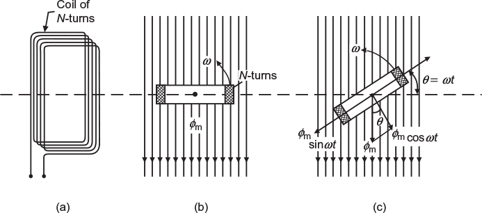
Fig. 6.6  Multi-turn coil rotating in a constant magnetic field (a) Multi-turn coil (b) Position of coil at an instant (c) Position of coil after t second

According to Faraday’s laws of electromagnetic induction, the magnitude of emf induced in the coil at this instant, that is,

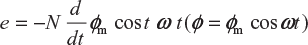
Instantaneous value of emf induced in the coil,

 (negative sign indicates that an induced emf is opposite to the very cause which produces it)

or

or

 

e = − N ɸ_m (−ω sin ω t)

or

 

e = ω N ɸ_m sin ω t        (6.1)

The value of an induced emf will be maximum when angle q

or

 

ωt = 90° (i.e., sin ωt = 1)

∴

 

E_m = ωNɸ_m        (6.2)

Putting this value in equation (6.1), we get,

 

e = E_m sin ωt = E_m sin θ

From the above equation, it is clear that the magnitude of the induced emf varies according to sine of angle θ. The wave shape of an induced emf is shown in Figure 6.7. This wave form is called sinusoidal wave.

If this voltage is applied across resistor, an alternating current will flow through it varying sinusoidally, that is, following a sine law and its wave shape will be same as shown in Figure 6.7.

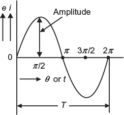
Fig. 6.7  Wave shape of a sinusoidal voltage or current

This alternating current is given by the following equation:

 

i = I_m sin ωt = I_m sin θ

6.7  IMPORTANT TERMS

An alternating voltage or current changes its magnitude and direction at regular intervals of time. A sinusoidal voltage or current varies as a sine function of time t or angle θ ( = ω t). The following important terms are generally used in alternating quantities:

1. Wave form: The shape of the curve obtained by plotting the instantaneous values of alternating quantity (voltage or current) along Y-axis and time or angle (θ = ωt) along X-axis is called ‘wave form or wave shape’. Figure 6.7 shows the waveform of an alternating quantity varying sinusoidally.
2. Instantaneous value: The value of an alternating quantity, that is, voltage or current at any instant is called its instantaneous value and is represented by ‘e’ or ‘i’, respectively.
3. Cycle: When an alternating quantity goes through a complete set of positive and negative values or goes through 360 electrical degrees, it is said to have completed one cycle.
4. Alternation: One half-cycle is called ‘alternation’. An alternation spans 180 electrical degrees.
5. Time period: The time taken in seconds to complete one cycle by an alternating quantity is called time period. It is generally denoted by ‘T’.
6. Frequency: The number of cycles made per second by an alternating quantity is called ‘frequency’. It is measured in cycles per second (c/s) or hertz (Hz) and is denoted by ‘f ’.
7. Amplitude: The maximum value (positive or negative) attained by an alternating quantity in one cycle is called its ‘amplitude or peak value or maximum value’. The maximum value of voltage and current is generally denoted by E_m (or V_m) and I_m, respectively.