
Information theory involves communication in general—on wires, fibers, or over the air—and it’s applied to widely varied applications such as information storage on optical disks, radar target identification, and the search for extraterrestrial intelligence. In general, the goal of a communication system is to pass “information” from one place to another through a medium contaminated by noise, at a particular rate, and at a minimum specified level of fidelity to the source. Information theory gives us the means for quantitatively defining our objectives and for achieving them in the most efficient manner. The use of radio as a form of communication presents obstacles and challenges that are more varied and complex than a wired medium. A knowledge of information theory lets us take full advantage of the characteristics of the wireless interface.
In order to understand what information theory is about, you need at least a basic knowledge of probability. We’ve already encountered uses of probability theory in this book—in comparing different transmission protocols and in determining path loss with random reflections.
The use of coding algorithms is very common today for highly reliable digital transmission even with low signal-to-noise ratios. Error correction is one of the most useful applications of information theory.
Finally, information theory teaches us the ultimate limitations in communication—the highest rate that can be transmitted with a given bandwidth and a given signal-to-noise ratio.
19.8.1 Probability
19.8.1.1 Basics
A common use of probability theory in communication is in assessing the reliability of a received message transmitted over a noisy channel. Let’s say we send a digital message frame containing 32 data bits. What is the probability that the message will be received in error—that is, that one or more bits will be corrupted? If we are using or are considering using an error-correcting code that can correct one bit, then we will want to know the probability that two or more bits will be in error. Another interesting question: what is the probability of error of a frame of 64 bits, compared to that of 32 bits, when the probability of error of a single bit is the same in both cases?
In all cases we must define what is called an experiment in probability theory. This involves defining outcomes and events and assigning probability measures to them that follow certain rules.
We state here the three axioms of probability, which are the conditions for defining probabilities in an experiment with a finite number of outcomes. We also must describe the concept of field in probability theory. Armed with the three axioms and the conditions of a field, we can assign probabilities to the events in our experiments. But, first, let’s look at some definitions.
An outcome is a basic result of an experiment. For example, throwing a die has six outcomes, each of which is a different number of dots on the upper face of the die when it comes to rest. An event is a set of one or more outcomes that has been defined, again according to rules, as a useful observation for a particular experiment. For an example, one event may be getting an odd number from a throw of a die and another event may be getting an even number. The outcomes are assigned probabilities and the events receive probabilities from the outcomes that they are made up of, in accordance with the three axioms. The term space refers to the set of all of the outcomes of the experiment. We’ll define other terms and concepts as we go along, after we list the three axioms.
Axioms of probability
I. P(A)≥0 The probability of an event A is zero or positive.
II. P(S)=1 The probability of space is unity.
III. If A .B=0 then P(A+B)=P(A)+P(B) If two events A and B are mutually exclusive, then the probability of their sum equals the sum of their individual probabilities.
The product of two events, shown in Axiom III as A .B and often called intersection, is an event which contains the outcomes that are common to the two events. The sum of two events A+B, also called union, is an event which contains all of the outcomes in both component events.
Mutually exclusive, referred to in Axiom III, means that two events have no outcomes in common. This means that if in an experiment one of the events occurs, the other one doesn’t. Returning to the experiment of throwing a die, the odd event and the even event are mutually exclusive.
Now we give the definition of a field, which tells us what events we must include in an experiment. We will use the term complement of an event, which is all of the outcomes in the space not included in the event. The complement of A is A´. A .A´ = 0.
Definition of a field F
If event A is contained in the field F, then its complement is also contained in F.
2. If A ∈F and B ∈F then A+B ∈F
If the events A and B are each contained in F, then the event that is the sum of A and B is also contained in F.
Now we need one more definition before we get back down to earth and deal with the questions raised and the uses mentioned at the beginning of this section.
Definition of independent events
Two events are called independent if the probability of their product (intersection) equals the product of their individual probabilities:

This definition can be extended to three or more events. For three independent events A, B, C:

Similarly, for more than three events the probability of the product of all events equals the product of the probabilities of each of the events, and the probability of the product of any lesser number of events equals the product of the probabilities of those events. If there are n independent events, then the total number of equations like those shown above for three events that are needed to establish their independence is:

19.8.1.2 Examples
We now can look at some examples of how to use probability theory.
Example 19.13
What is the probability of correctly receiving a sequence of 12 bits if the probability of error of a bit is one out of one hundred, or pe=.01? All bits are independent.
Solution
We look at the problem as an experiment in which we must define space, events according to the conditions of a field, and the probabilities of the events. We’ll call the probability of a correct sequence Pc and the probability of an error in the sequence Pe.
The space in our experiment contains all conceivable outcomes. Since we have a sequence of 12 bits, we can receive 212=4096 different sequences of bits, or words. The events in our experiment, conforming to the conditions for a field, are:
(1) The reception of the correct word—that is, no bits are in error.
(2) The reception of an erroneous word—a sequence that has 1 or more bits in error.
(3) The reception of any word.
The inclusion of event (3) is necessary because of condition 2 in the definition of a field, which says that the event that is the sum of events must also be in the field. The sum of events (1) and (2) is all of the outcomes, which is the space, and this is event (3). Event (4) is needed because of condition 1 of a field—the complement of any event must be included—and event (4) is the complement of event (3). The complements of events (1) and (2) are each other, so the requirements of a field are complied with.
Now we assign probabilities to the events. In the statement of the problem we designated the probability of a bit error as pe. In the field of an individual bit, we have two events: bit error or no bit error. The sum of these two events is the bit space, whose probability is unity. It follows that the probability of no bit error+probability of bit error (pe)=probability of space (1). Thus, the probability of no bit error=1 –pe.
Now, the bits in the received sequence are independent, so the probability of a particular sequence equals the product of the probabilities of each of its bits. In the case of the errorless sequence, the probability that each bit has no bit error is 1 –pe, so this sequence’s probability is (1 –pe)12. Using the given bit error probability of .01, we find that the probability of correctly receiving the sequence is .9912 or approximately 88.6 percent.
How can we interpret this answer? If the sequence is sent only once for all time, it will either be received correctly or it won’t. In this case, the establishment of a probability won’t have much significance, except for the purpose of placing bets. However, if sequences are sent repeatedly, we will find that as the number of sequences increases, the percentage of those correctly received approaches 88.6.
Just as we found the probability of no bit error=1 – pe, we find the probability of a sequence error is 1 – .886=0.114. This is from axioms II and III and the fact that the sum of the two mutually exclusive events—incorrect and correct sequences—is space, whose probability is 1.
Figure 19.30 gives a visual representation of this problem, showing space, the events, and the outcomes. Each outcome, representing one of the 4096 sequences, is assigned a probability Pi:

where p1, p2, and so on equals either pe or 1 –pe, depending on whether that specific bit in the sequence is in error or not. Sequences having the same number of error bits have identical probabilities.

Figure 19.30 A probability space
For example, an outcome that is a sequence having one bit in error has a probability of pe (1-pe)11. There are 12 of these mutually exclusive sequences, so the probability of receiving a sequence having one and only one error bit is:

19.8.1.3 Conditional Probability
An important concept in probability theory is conditional probability. It is defined as follows:
Given an event B with nonzero probability P(B)>0, then the conditional probability of event A assuming event B is known as:
![]() (19.21)
(19.21)
A consequence of this definition is that the probability of an event is affected by the assumption of occurrence of another event. We see from the expression above that if A and B are mutually exclusive, the conditional probability is zero because P(A .B)=0. If A and B are independent, then the occurrence of B has no effect on the probability of A : P(A|B)=P(A). Conditional probabilities abide by the three axioms and the definition of a field.
Up to now we have discussed only sets of finite outcomes, but the theory holds when events are defined in terms of a continuous quantity as well. A space can be the set of all real numbers, for example, and subsets, or events, to which we can assign probabilities are intervals in this space. For example, we can talk about the probability of a train arriving between 1 and 2 p.m., or of the probability of a received signal giving a detector output above 1 volt. The axioms and definition of a field still hold but we have to allow for the existence of infinite sums and products of events.
19.8.1.4 Density and Cumulative Distribution Functions
In the problem above we found the probability, in a sequence of 12 bits, of getting no errors, of getting an error (one or more errors), and of getting an error in one bit only. We may be interested in knowing the probability of receiving exactly two bits in error, or any other number of error bits. We can find it using a formula called the binomial distribution:
![]() (19.22)
(19.22)
where Pm(n) is the probability of receiving exactly n bits in error, m is the total number of bits in the sequence, p is the probability of one individual bit being in error and q=1-p, the probability that an individual bit is correct. ![]() represents the number of different combinations of n objects taken m at a time:
represents the number of different combinations of n objects taken m at a time:
The notation ! is factorial—for example, m!=m(m-1)(m-2) … (1).
Each time we send an individual sequence, the received sequence will have a particular number of bits in error—from 0 to 12 in our example. When a large number of sequences are transmitted, the frequency of having exactly n errors will approach the probability given in Eq. (19.22). In probability theory, the quantity that expresses the observed result of a random process is called a random variable. In our example, we’ll call this random variable N. Thus, we could rewrite Eq. (19.22) as:
![]() (19.22a)
(19.22a)
(We represent uppercase letters as random variables and lowercase letters as real numbers. We may write P(x) which means the probability that random variable X equals real number x.)
The random value can be any number that expresses an outcome of an experiment, in this case 0 through 12. The random values are mutually exclusive events.
The probability function given in Eq. (19.22a), which gives the probability that the random variable equals a discrete quantity, is sometimes called the frequency function. Another important function is the cumulative probability distribution function, or distribution function, defined as:
![]() (19.23)
(19.23)
defined for any number x from -∞ to +∞ and X is the random value.
In our example of a sequence of bits, the distribution function gives the probability that the sequence will have n or fewer bits in error, and its formula is
![]() (19.24)
(19.24)
where Σ is the symbol for summation.
The example which we used up to now involves a discrete random variable, but probability functions also relate to continuous random variables, such as time or voltage. The best known of these is probably the Gaussian probability function, which describes, for example, thermal noise in a radio receiver. The analogous type of function to the frequency probability function defined for the discrete variable is called a density function. The Gaussian probability density function is:
![]() (19.25)
(19.25)
where σ2 is the variance and m is the average (defined below).
Plots of the frequency function Pm(n) (p and q=1/2) and the density function P(x), with the same average and variance, are shown in Figure 19.31. While these functions are analogous, as stated above, there are also fundamental differences between them. For one, P(x) is defined on the whole real abscissa, from -∞ (infinity) to +∞ whereas Pm(n) can have only the discrete values 0 to 12. Second, points on P(x) are not probabilities! A continuous random variable can have a probability greater than zero only over a finite interval. Thus, we cannot talk about the probability of an instantaneous noise voltage of 2 V, but we can find the probability of it being between, say, 1.8 and 2.2 V. Probabilities on the curve P(x) are the area under the curve over the interval we are interested in. We find these areas by integrating the density curve between the endpoints of the interval, which may be plus or minus infinity.
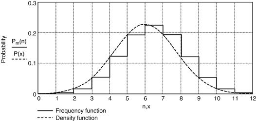
Figure 19.31 Frequency and density functions
The more useful probability function for finding probabilities directly for continuous random variables is the distribution function. Figure 19.30 shows the Gaussian distribution function, which is the integral of the density function between -∞ and x. All distribution functions have the characteristics of a positive slope and values of 0 and 1 at the extremities. To find the probability of a random variable over an interval, we subtract the value of the distribution function evaluated at the lower boundary from its value at the upper boundary. For example, the probability of the interval of 4 to 6 in Figure 19.32 is:


Figure 19.32 Gaussian distribution function
19.8.1.5 Average, Variance, and Standard Deviation
While the distribution function is easier to work with when we want to find probabilities directly, the density function or the frequency function is more convenient to use to compute the statistical properties of a random variable. The two most important of these properties are the average and the variance.
The statistical average for a discrete variable is defined as:
![]() (19.26)
(19.26)
Writing this using the frequency function for the m-bit sequence (Eq. (19.2)) we have:
where n ranges from 0 to m.
Calculating the average using p=.1, for example, we get ![]() bits. In other words, the average number of bits in error in a sequence with a bit error probability of .1 is just over 1 bit.
bits. In other words, the average number of bits in error in a sequence with a bit error probability of .1 is just over 1 bit.
The definition of the average of a continuous random variable is:
![]() (19.27)
(19.27)
If we apply this to the expression for the Gaussian density function in Eq. (19.5) we get ![]() as expected.
as expected.
We can similarly find the average of a function of a random variable, in both the discrete and the continuous cases:
When this function is expressed as f(x)=xn, its average is called the nth moment of X. The first moment of X is its average, shown above. The second moment of the continuous random variable x is:
![]() (19.28)
(19.28)
In the case where the random variable has a nonzero average, a, a more useful form of the second moment is the second-order moment about a point a, also called the second-order central moment, defined as:
![]() (19.29)
(19.29)
The second-order central moment of X is called the variance of X, and its square root is the standard deviation. The standard deviation, commonly represented by the Greek letter sigma (σ), gives a measure of the form factor of a probability density function. Figure 19.33 shows two Gaussian density functions, one with s=1 and the other with s=2. Both have the same average, m.

Figure 19.33 Gaussian density function with different standard deviations
The first and second moments are used all the time by electrical engineers when they are talking about voltages and currents, either steady-state or random. The first moment is the DC level and the second moment is proportional to the power. The variance of a voltage across a unit resistance is its AC power, and the standard deviation is the RMS value of a current or voltage about its DC level.
19.8.2 Information Theory
In 1948 C. E. Shannon published his Mathematical Theory of Communication, which was a tremendous breakthrough in the understanding of the possibilities of reliable communication in the presence of interference. A whole new field of study opened up, that of information theory, which deals with three basic concepts: the measure of information, the capacity of a communication channel to transfer information, and the use of coding as the means of approaching error-free communication at rates that approach this capacity. Much of the significance of Shannon’s work can be realized by considering this statement, which sums up what is called the fundamental theorem of information theory:
It is possible to transmit information through a noisy communication channel at any rate up to the channel capacity with an arbitrarily small probability of error.
The converse of this statement has also been proven:
It is not possible to achieve reliable communication through a channel at a rate higher than the channel capacity.
The key to reliable communication in the presence of noise is coding. We will look at an example of error correction coding after a brief review of the basics of information theory.
19.8.2.1 Uncertainty, Entropy, and Information
Engineers generally talk about bit rate as the number of binary symbols that are transmitted per unit time. In information theory, the bit has a different, deeper meaning. Imagine the transmission of an endless stream of digital ones where each one has a duration of one millisecond. Is the rate of communication 1000 bits/second? According to information theory, the rate is zero. A stream of ones, or any other repetitive pattern of symbols reveals nothing to the receiver, and even in the presence of noise and interference, the “message” is always detected with 100 percent certainty. The more uncertain we are about what is being transmitted, the more information we get by correctly receiving it. In information theory, the term bit is a unit used to measure a quantity of information or uncertainty.
Information theory defines mathematically the uncertainty of a message or a symbol. Let’s say we want to send a message using a sequence of three binary digits. We know that we can send up to eight different messages using this sequence (23). Each message has a particular probability of being sent. An example of this situation is a room with 8 patients in a hospital that has a nurse call system. When one of the patients presses a button next to his or her bed, a three-digit message is sent to the nurse’s desk where it rings a bell and causes a display to show a number representing that patient. Depending on their condition, some patients may use the call system more than others. We present the probability of a patient pressing the nurse call button in Table 19.1.
Table 19.1
Data for example
| Patient’s Name | Patient’s Number | Probability |
| John | 1 | .1 |
| Mary | 2 | .5 |
| Jane | 3 | .2 |
| Mike | 4 | .05 |
| Pete | 5 | .05 |
| Sue | 6 | .03 |
| Tom | 7 | .01 |
| Elaine | 8 | .06 |
The total probability of one of them having pressed the call button when the bell rings is, of course, 1.
When the nurse hears the bell, she won’t be surprised to see the number 2 on the display, since Mary requires assistance more than any of the other patients. The display of “7” though will be quite unexpected, since Tom rarely resorts to calling the nurse. The message indicating that Tom pressed his assistance button gives more information than the one triggered by Mary.
If we label the probability of an event, such as a patient pressing the assistance button, by pi, we quantify the self-information of the event i by:
![]() (19.30)
(19.30)
With i referring to the number of the patient, we find that the self information of Mary’s signal is I(2)=log2(2)=1 bit, and Tom’s signal self-information is I(7)=log2(100)=6.64 bits. The unit of self-information is the bit when the log is taken to the base 2. The self-information of the other patients’ signals can be found similarly.
More important than the individual self-information of each of the signals is the average self-information of all the signals. This quantity is commonly labeled H and is called the uncertainty of the message, or its entropy. The latter term was taken from a value in thermodynamics with similar properties. Taking the statistical average of the self information, we get:
![]() (19.31)
(19.31)
With i ranging from 1 to 8 and using the probabilities in the table above, we get for our present example:


Now let’s assume that all of the patients are equally likely to call the nurse. The self-information of each signal I(i) in this case is log2(8)=3 bits. The entropy is:

It turns out that this is the maximum possible entropy of the message—the case where the probability of each of the signals is equal.
Let’s stretch our example of the nurse call system to an analogy with a continuous stream of binary digits. We’ll assume the patients press their call buttons one after another at a constant rate.
In the case where the signal probabilities are distributed as in the table, the entropy per digit is H/3=.73. If each patient pressed his button with equal probability, the entropy per digit would be the maximum of Hm/3=1. So with the different probabilities as listed in the table, the system communicates only 73% of the information that is possible to send over the communication channel per unit time. Using coding, discussed below, we can match a source to a channel to approach the channel’s capability, or capacity, to any extent that we want it to.
Up to now we have been talking about the entropy, or uncertainty, of a source, and have assumed that what is sent is what is received. At least of equal importance is to measure the entropy, and the information, involved with messages sent and received over a noisy channel. Because of the noise, the probabilities of the received messages might not be the same as those of the source messages, because the receiver will make some wrong decisions as to the identity of the source. We saw above that entropy is a function of probabilities, and in the case of communication over a noisy channel, several sets of probability functions can be defined.
On a discrete, memoryless channel (memoryless because the noise affecting one digit is independent of the noise affecting any other digit) we can present the effect of the noise as a matrix of conditional probabilities. Assume a source transmits symbols having one of four letters x1, x2, x3, and x4. X is a random variable expressing the transmitted symbol and Y is a random variable for the received symbol. If a symbol x1 happens to be sent, the receiver may interpret it as y1, y2, y3, or y4, depending on the effect of the random noise at the moment the symbol is sent. There is a probability of receiving y1 when x1 is sent, another probability of receiving y2 when x1 is sent, and so on for a matrix of 16 probabilities as shown below:
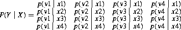 (19.32)
This example shows a square matrix, which means that the receiver will interpret a signal as being one of those letters that it knows can be transmitted, which is the most common situation. However, in the general case, the receiver may assign a larger or smaller number of letters to the signal so the matrix doesn’t have to be square.
The conditional entropy of the output Y when the input X is known is:
![]() (19.33)
(19.33)
where the sums are over the number of source letters xi and received letters yj, and to get units of bits the log is to the base 2. The expression has a minus sign to make the entropy positive, canceling the sign of the log of a fraction, which is negative.
If we look only at the Ys that are received, we get a set of probabilities p(y1) through p(y4), and a corresponding uncertainty H(Y).
Knowing the various probabilities that describe a communication system, expressed through the entropies of the source, the received letters, and the conditional entropy of the channel, we can find the important value of the mutual information or transinformation of the channel. In terms of the entropies, we defined above:
![]() (19.34a)
(19.34a)
The information associated with the channel is expressed as the reduction in uncertainty of the received letters given by a knowledge of the statistics of the source and the channel. The mutual information can also be expressed as:
![]() (19.34b)
(19.34b)
which shows the reduction of the uncertainty of the source by the entropy of the channel from the point of view of the receiver. The two expressions of mutual information are equal.
19.8.2.2 Capacity
In the fundamental theorem of information theory, summarized above, the concept of channel capacity is a key attribute. It is connected strongly to the mutual information of the channel. In fact, the capacity is the maximum mutual information that is possible for a channel having a given probability matrix:
![]() (19.35)
(19.35)
where the maximization is taken over all sets of source probabilities. For a channel that has a symmetric noise characteristic, so that the channel probability matrix is symmetric, the capacity is easily shown to be:
![]() (19.36)
(19.36)
where m is the number of different letters for each source symbol and h=H(Y|X), a constant independent of the input distribution when the channel noise is symmetric. This is the case for expression (19–12), when each row of the matrix has the same probabilities except in different orders.
For the noiseless channel, as in the example of the nurse call system, the maximum information that could be transferred was Hm=3 bits/ message, achieved when the source messages all have the same probability. Taking that example into the frame of the definition of capacity, Eq. (19.36), the number of different messages is the number of letters per symbol, so for m=8 (“messages”):
![]() (19.36a)
(19.36a)
This is a logical extension of the more general case presented previously. Here the constant h=0 for the situation when there is no noise.
Another situation of interest for finding capacity on a discrete memoryless channel is when the noise is such that the output Y is independent of the input X, and the conditional entropy H(Y|X)=H(Y). The mutual information of such a channel I(X;Y)=H(Y) –H(Y|X)=0 and the capacity is also zero.
The notion of channel capacity and the fundamental theorem also hold for continuous, “analog” channels, where signal-to-noise ratio (S/N) and bandwidth (B) are the characterizing parameters. The capacity in this case is given by the Hartley-Shannon law:
![]() (19.37)
(19.37)
The extension from a discrete system to a continuous one is easy to conceive of when we consider that a continuous signal can be converted to a discrete one by sampling, where the sampling rate is a function of the signal bandwidth (at least twice the highest frequency component in the signal).
From a glance at (19–17) we easily see that bandwidth can be traded off for signal-to-noise ratio, or vice-versa, while keeping a constant capacity. Actually, it’s not quite that simple since the signal-to-noise ratio itself depends on the bandwidth. We can show this relationship by rewriting (19.17) using n=the noise density. Substituting N=n.B:
![]() (19.38)
(19.38)
In this expression the tradeoff between bandwidth and signal-to-noise ratio (or transmitter power) is tempered somewhat but it still exists. This doesn’t mean that increasing the bandwidth automatically lets us send a higher data rate and keep a low probability of errors. We must use coding to keep the error rate down, but the higher bandwidth facilitates the addition of error-correcting bits in accordance with the coding algorithm.
In radio communication, a common aim is the reduction of signal bandwidth. Shannon-Hartley indicates that we can reduce bandwidth if we increase signal power to keep the capacity constant. This is fine, but Figure 19.34 shows that as the bandwidth is reduced more and more below the capacity, large increases in signal power are needed to maintain that capacity.

Figure 19.34 Signal power vs. bandwidth at constant capacity
19.8.2.3 Coding
We can represent a communication system conveniently by the block diagram in Figure 19.35. Assume the source outputs binary data, although if it were analog, we could make it binary by passing it through an analog-to-digital converter. The modulator and demodulator act as interfaces between the discrete signal parts of the system and the waveform that passes information over the physical channel—the modulated carrier frequency in a wireless system, for example.

Figure 19.35 Communication system
We can take the modulator and demodulator blocks together with the channel and its noise input and look at the ensemble as a binary discrete channel. Consider the encoder and decoder blocks as matching networks which process the binary data so as to get the most “power” out of the system, in analogy to a matching network that converts the RF amplifier output impedance to the conjugate impedance of the antenna in order to get maximum power transfer. “Power,” in the case of the communication link, may be taken to mean the data rate and the equivalent probability of error. A perfect match of the encoder and decoder to the channel gives a rate of information transfer equaling the capacity of the equivalent binary channel with an error rate approaching zero.
19.8.2.4 Noiseless Coding
When there’s no noise in the channel (or relatively little) there is no problem of error rate but coding is still needed to get the maximum rate of information transfer. We saw above that the highest source entropy is obtained when each message has the same probability. If source messages are not equi-probable, then the encoder can determine the message lengths that enter the binary channel so that highly probable messages will be short, and less probable messages will be long. On the average, the channel rate will be obtained.
For example, let’s say we have four messages to send over a binary channel and that their rates of occurrence (probabilities) are 1/2, 1/4, 1/8, and 1/8. Table 19.2 shows two coding schemes that may be chosen for the messages m1, m2, m3, and m4.
Table 19.2
Two coding schemes
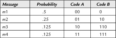
One of the possible streams of messages that represents the probabilities is m1 .m1 .m1 .m1 .m2 .m2 .m3 .m4. The bit streams that would be produced by each of the two codes is:
Code A needs 16 binary symbols, or digits, to send the message stream while Code B needs only 14 digits. Thus, using Code B, we can make better use of the binary channel than if we use Code A, since, on the average, it lets us send 14% more messages using the same digit rate.
We can determine the best possible utilization of the channel by calculating the entropy of the messages, which is (from 19.11 above):


In the example, we sent 8 messages, which can be achieved using a minimum of 8×H=14 digits, where each digit carries one bit of information. This we get using Code B.
The capacity of the binary symmetric channel, which sends ones and zeros with equal probability, is (from Eq. 19.16):

Each digit on the channel is a bit, so Code B fully utilizes the channel capacity. If each message had equal probability, H would be log2(4)=2 bits per message. Then the best code to use would be code A. You can prove it yourself using a message stream with each message occurring an equal number of times and checking how many digits you need for each code. The point is that the chosen code matches the entropy of the source to get the maximum rate of communication.
There are several schemes for determining an optimum code when the message probabilities are known. One of them is Huffman’s minimum-redundancy code. This code, like the one in the example above, is easy to decode because each word in the code is distinguishable without a deliminator and decoding is done “on the fly.” When input probabilities are not known, such codes are not applicable. An example of a code that works on a bit stream without dependency on source probabilities or knowledge of word lengths is the Lempel-Ziv algorithm, used for file compression. Its basic idea is to look for repeated strings of characters and to specify where a previous version of the string started and how many characters it has.
The various codes used to transfer a given amount of “information” in the shortest time for a given bit rate are often called compression schemes, since they also can be viewed as reducing the number of symbols, or bits, needed to represent this information. One should remember that when the symbols in the input message stream are randomly distributed, coding will not make any difference from the point of view of compression or increasing the message transmission rate.
19.8.2.5 Error Detection and Correction
A most important use of coding is on noisy channels where you want to reduce the error rate while maintaining a given message transmission rate. We’ve already learned from Shannon that it’s theoretically possible to reduce the error rate to as close to zero as we want, as long as the signal rate is below channel capacity. There’s more than one way to look at the advantage of coding for error reduction. For example, if we demand a given maximum error rate in a communication system, we can achieve that goal without coding by increasing transmitter power to raise the signal-to-noise ratio and thereby reduce errors. We can also reduce errors by reducing the transmission rate, allowing us to reduce bandwidth, which will also improve the signal-to-noise ratio (since noise power is proportional to bandwidth). So using coding for error correction lets us either use lower power for a given error rate, or increase transmission speed for the same rate. The reduction in signal-to-noise ratio that can be obtained through the use of coding to achieve a given error rate compared to the signal-to-noise ratio required without coding for the same error rate is defined as the coding gain.
A simple and well-known way to increase transmission reliability is to add a parity bit at the end of a block, or sequence, of message bits. The parity bit is chosen to make the number of bits in the message block odd or even. If we send a block of seven message bits, say 0110110, and add an odd parity bit, and the receiver gets the message 01001101, it knows that the message has been corrupted by noise, although it doesn’t know which bit is in error. This method of error detection is limited to errors in an odd number of bits, since if, say, two bits were corrupted, the total number of bits is still odd and the errors are not noticed. When the probability of a bit error is relatively low, by far most errors will be in one bit only, so the use of one parity bit may still be useful.
Another simple way to provide error detection is by logically adding together the contents of a number of message blocks and appending the result as an additional block in the message sequence. The receiver performs the same logic summing operation as the transmitter and compares its computation result to the block appended by the transmitter. If the blocks don’t match, the receiver knows that one or more bits in the message blocks received are not correct. This method gives a higher probability of detection of errors than does the use of a single parity bit, but if an error is detected, more message blocks must be rejected as having suspected errors.
When highly reliable communication is desired, it’s not enough just to know that there is an error in one or more blocks of bits, since the aim of the communication is to receive the whole message reliably. A very common way to achieve this is by an automatic repeat query (ARQ) protocol. After sending a message block, or group of blocks, depending on the method of error detection used, the transmitter stops sending and listens to the channel to get confirmation from the receiver. After the receiver notes that the parity bit or the error detection block indicates no errors, it transmits a short confirmation message to the transmitter. The transmitter waits long enough to receive the confirmation. If the message is confirmed, it transmits the next message. If not, it repeats the previous message.
ARQ can greatly improve communication reliability on a noisy communication link. However, there is a price to pay. First, the receiver must have a transmitter, and the transmitter a receiver. This is OK on a two-way link but may be prohibitive on a one-way link such as exists in most security systems. Second, the transmission rate will be reduced because of the necessity to wait for a response after each short transmission period. If the link is particularly noisy and many retransmissions are required, the repetitions themselves will significantly slow down the communication rate. In spite of its limitations, ARQ is widely used for reliable communications and is particularly effective when combined with a forward error correction scheme as discussed in the next section.
19.8.2.6 Forward Error Correction (FEC)
Just as adding one odd or even parity bit allows determining if there has been an error in reception, adding additional parity bits can tell the location of the error. For example, if the transmitted message contains 15 bits, including the parity bits, the receiver will need enough information to produce a four-bit word to indicate that there are no errors, (error word 0000), or which bit is in error (one out of 15 error words 0001 through 1111). The receiver might be able to produce this four-bit error detection and correction word from four parity bits (in any case, no less than four parity bits), and then we could send 11 message information bits plus four parity bits and get a capability of detecting and correcting an error in any one bit.
R.W. Hamming devised a relatively simple method of determining parity bits for correcting single-bit errors. If n is the total number of message bits in a sequence to be transmitted, and k is the number of parity bits, the relationship between these numbers permitting correction of one digit is:
![]() (19.39)
(19.39)
If we represent m as the number of information bits (n=m+k) we can find n and k for several values of m in Table 19.3.
Table 19.3
Values of m, n, and k
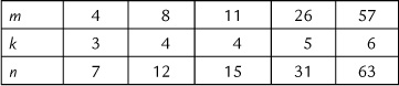
As an example, one possible set of rules for finding the four parity bits for a total message length of 12 bits (8 information bits), derived from Hamming’s method, is as follows.
We let x1, x2, x3, and so on, represent the position of the bits in the 12-bit word. Bits x1, x2, x4, and x8 are chosen in the transmitter to give even parity when the bits are summed up using binary arithmetic as shown in the four equations below (in binary arithmetic, 0+0=0, 0+1=1, 1+0=1, 1+1=0). Let s1 through s4 represent the results of the equations.
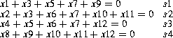
In this scheme, x1, x2, x4, and x8 designate the location of the parity bits. If we number the information bits appearing, say, in a byte-wide register of a microcomputer, as m1 through m8, and we label the parity bits p1 through p4, then the transmitted 12-bit code word would look like this:

Those parity bits are calculated by the transmitter for even parity as shown in the four equations.
When the receiver receives a code word, it computes the four equations and produces what is called a syndrome—a four-bit word composed of s4 .s3 .s2 .s1. .s1 is 0 if the first equation=0 and 1 otherwise, and so on for s2, s3, and s4. If the syndrome word is 0000, there are no single-bit errors. If there is a single-bit error, the value of the syndrome points to the location of the error in the received code word, and complementing that bit performs the correction. For example, if bit 5 is received in error, the resulting syndrome is 0101, or 5 in decimal notation (you should check this by calculating the equations).
Note that different systems could be used to label the code bits. For example, the four parity bits could be appended after the message bits. In this case a lookup table might be necessary in order to show the correspondence between the syndrome word and the position of the error in the code word.
The one-bit correcting code just described gives an order of magnitude improvement of message error rate compared to transmission of information bytes without parity digits, when the probability of a bit error on the channel is 10-2. However, one consequence of using an error-correcting code is that, if message throughput is to be maintained, a faster bit rate on the channel is required, which entails reduced signal-to-noise ratio because of the wider bandwidth needed for transmission. This rate, for the above example, is 12/8 times the uncoded rate, an increase of 50%. Even so, there is still an advantage to coding, particularly when coding is applied to larger word blocks.
Error probabilities are usually calculated on the basis of independence of the noise from bit to bit, but on a real channel, this is not likely to be the case. Noise and interference tend to occur in bursts, so several adjacent bits may be corrupted. One way to counter the noise bursts is by interleaving blocks of code words. For simplicity of explanation, let’s say we are using four-bit code words. Interleaving the code words means that after forming each word with its parity bits in the encoder, the transmitter sends the first bit of the first word, then the first bit of the second word, and so on. The order of transmitted bits is best shown as a matrix, as in Table 19.4, where the as are the bits of the first word, and b, c, and d represent the bits of the second, third, and fourth words.
Table 19.4
Matrix showing order of transmitted bits
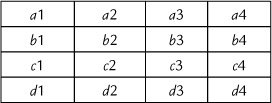
The order of transmission of bits is a1 .b1 .c1 .d1 .a2 .b2 …d3 .a4 .b4 .c4 .d4. In the receiver, the interleaving is decomposed, putting the bits back in their original order, after which the receiver decoder can proceed to perform error detection and correction.
The result of the interleaving is that up to four consecutive bit errors can occur on reception and the decoder can still correct them using a one-bit error correcting scheme. A disadvantage is that there is an additional delay of three word durations until decoded words start appearing at the destination.
Forward error correction schemes which deal with more than one error per block are much more complicated, and more effective, than the Hamming code described here. An important class of codes which are not based on blocks of bits but rather add parity bits based on logic operations on a small number of previous bits is called convolutional codes. In general, coding is a very important aspect of radio communication and its use and continued development is a prime reason why radio communication can continue to replace wires while making more effective use of the available spectrum and limited transmitter power.
19.8.3 Summary of Probability and Coding Principles
In this chapter we reviewed the basics of probability and coding. Sets of probabilities were applied both to the different signals generated by the source, as well as to the characteristics of a communication channel corrupted by noise. We saw that associated with a noisy communication channel is a maximum data rate called the capacity of the channel.
Through the use of coding, which involves inserting a redundancy in the transmitted data, it’s possible to approach error-free communication up to the capacity of the channel.
Although effective and efficient coding algorithms are quite complicated, the great advances in integrated circuit miniaturization and logic circuit speed in recent years have allowed incorporating error-correction coding in a wide range of wireless communications applications. Many of these applications are in products that are mass produced and relatively low cost—among them cellular telephones and wireless local area networks. This trend will certainly continue and will give even the most simple short-range wireless products “wired” characteristics from the point of view of communication reliability.
This chapter has discussed matters which are not necessarily limited to radio communication, and where they do apply to radio communication, not necessarily to short-range radio. However, anyone concerned with getting the most out of a short-range radio communication link should have some knowledge of information theory and coding. The continuing advances in the integration of complex logic circuits and digital signal processing are bringing small, battery-powered wireless devices closer to the theoretical bounds of error-free communication predicted by Shannon fifty years ago.
Leave a Reply