
As a practical example of the power of DSP, consider the comparison between an analog and a digital low-pass filter, each with a cutoff frequency of 1 kHz. The digital filter is implemented in a typical sampled data system shown in Figure 16.4. Note that there are several implicit requirements in the diagram. First, it is assumed that an ADC/ DAC combination is available with sufficient sampling frequency, resolution, and dynamic range to accurately process the signal. Second, the DSP must be fast enough to complete all its calculations within the sampling interval, 1/fs. Third, analog filters are still required at the ADC input and DAC output for antialiasing and anti-imaging, but the performance demands are not as great. Assuming these conditions have been met, the following offers a comparison between the digital and analog filters.
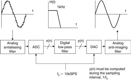
Figure 16.4 Digital filter
The required cutoff frequency of both filters is 1 kHz. The analog filter is realized as a 6-pole Chebyshev Type 1 filter (ripple in pass band, no ripple in stop band), and the response is shown in Figure 16.5. In practice, this filter would probably be realized using three 2-pole stages, each of which requires an op amp, and several resistors and capacitors. Modern filter design CAD packages make the 6-pole design relatively straightforward, but maintaining the 0.5 dB ripple specification requires accurate component selection and matching.
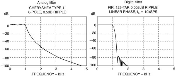
Figure 16.5 Analog versus digital filter frequency response comparison
On the other hand, the 129-tap digital FIR filter shown has only 0.002 dB pass band ripple, linear phase, and a much sharper roll-off. In fact, it could not be realized using analog techniques. Another obvious advantage is that the digital filter requires no component matching, and it is not sensitive to drift since the clock frequencies are crystal controlled. The 129-tap filter requires 129 multiply-accumulates (MAC) in order to compute an output sample. This processing must be completed within the sampling interval, 1/fs, in order to maintain real-time operation. In this example, the sampling frequency is 10 kSPS; therefore 100 μs is available for processing, assuming no significant additional overhead requirement. The ADSP-21xx family of DSPs can complete the entire multiply-accumulate process (and other functions necessary for the filter) in a single instruction cycle. Therefore, a 129-tap filter requires that the instruction rate be greater than 129/100 μs=1.3 million instructions per second (MIPS). DSPs are available with instruction rates much greater than this, so the DSP certainly is not the limiting factor in this application. The ADSP-218x 16-bit fixed-point series offers instruction rates up to 75 MIPS.
The assembly language code to implement the filter on the ADSP-21xx family of DSPs is shown in Figure 16.6. Note that the actual lines of operating code have been marked with arrows; the rest are comments.
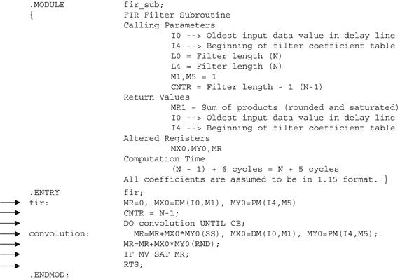
Figure 16.6 ADSP-21xx FIR filter assembly code (single precision)
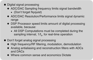
In a practical application, there are certainly many other factors to consider when evaluating analog versus digital filters, or analog versus digital signal processing in general. Most modern signal processing systems use a combination of analog and digital techniques in order to accomplish the desired function and take advantage of the best of both the analog and the digital worlds.{{{FIGURE 16.7}}}
Leave a Reply