Support Vector Machine (SVM)

A support vector machine (SVM) is a classification algorithm that classifies data based on its features. An SVM will classify any new element into one of the two classes as shown in Fig. 2.36.

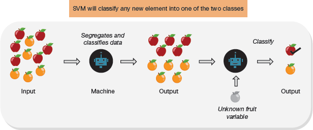
FIGURE 2.36 Classification Process using SVM

To make our machine learning model learn, we supply input data to it. The SVM algorithm will automatically extract features from the input data. This knowledge is used to segregate and classify the input data to generate the desired output. Once the model has learnt how to classify, any new data inputted to it can be classified (with a specific accuracy).

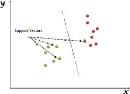
FIGURE 2.37 Identifying Best Line on the Plot for Classification

An SVM is therefore a supervised machine learning algorithm which can be used for both classification or regression challenges. However, it is mostly used to classify data. In the SVM algorithm, each data item is plotted as a point in n-dimensional space (where n is number of features). In this plot, support vectors are simply the co-ordinates of individual observation. For classification, we need to identify the best hyper plane/line or class (refer Fig. 2.37). For example, consider the scenarios given below.

Scenario 1: In Fig. 2.38, there are three hyper planes A, B and C. However, hyper planes B and C better segregates the two classes.

Scenario 2: When all three hyper-planes (A, B and C) are segregating the classes well, we must choose one that maximizes the distances between nearest data point (either class) and hyper-plane. This distance is called margin.

 

Note: Hyper plane with low margin can result in mis-classification.

In Fig. 2.38, we see that the margin for hyper-plane C is high as compared to both A and B. Hence, hyper plane C is chosen as the right decision boundary or hyper plane.

Scenario 3: In this scenario, hyper plane A is selected as it maximizes the margin and reduces classification error.

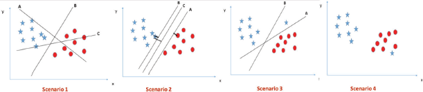
FIGURE 2.38 Identifying Hyperplanes on the Plot for Classification

Scenario 4: In Fig. 2.38, segregation is difficult as one star lies in the territory of circle class.

Scenario-5: In the scenario, linear hyper-plane between the two classes is not possible. However, SVM can solve this solution in two ways.

Solution 1: Adding a new feature z=x^2+y^2 and plotting the data points on axis x and z.

In the plot,

1. all values for z would be positive always because z is the squared sum of both x and y
2. In the original plot, red circles appear close to the origin of x and y axes because of lower value of z. Stars appear away from the origin due to higher value of z.

Solution 2: Use the kernel trick of the SVM algorithm. The SVM kernel is a function that takes low dimensional input space and transforms it to a higher dimensional space, that is, it converts not separable problem to separable problem. It is usually used in non-linear separation problem. In the figure, we see that the hyper-plane in original input space looks like a circle.

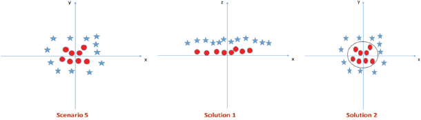
FIGURE 2.39 Evaluating Hyperplanes

Example:

Cricket players can be classified as batsmen or bowlers using the runs-to-wicket ratio. A player with more runs is a batsman and the one with more wickets is a bowler.

In this example (refer Fig. 2.40), we can create a two-dimensional plot showing a clear separation between bowlers and batsmen.

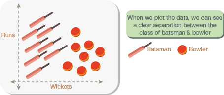
FIGURE 2.40 2D Plot representing Batsmen and Bowlers Data

Whenever we get data for a new player that is not yet classified, we draw a decision boundary, or a line separating the two classes to help classify the new data points. We can draw multiple decision boundaries as shown in Fig. 2.41. Therefore, the aim is to find the line of best fit that clearly separates those two groups. The correct line will help to classify the new data point.

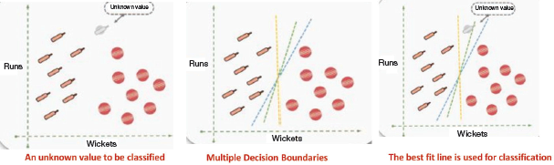
FIGURE 2.41 Identifying Line of Best Fit

The best fit line is computed by evaluating the maximum margin from equidistant support vectors. Support vectors mean two points (one from each class) that are closest together, but that maximize the distance between them or the margin.

Points to Remember

1. Hyperplane is a line in 2D, plane in 3D and hyper plane in higher dimensions (above 3 dimensions).
2. Margin is the distance between the hyperplane and the closest data point. We need to maximize this margin for better classification.
3. The kernel function is used to handle non-linear separable data. It does this by transforming data into a higher dimensional feature space to make it possible to perform the linear separation. Different kernel functions include the following:
   1. Gaussian RBF kernel
   2. Sigmoid kernel
   3. Polynomial kernel

Any of these functions can be chosen depending on the dimensions and way data has to be transformed.

Tuning Parameters

Tuning parameters can be divided into two groups—linear kernel SVM and non-linear kernel SVM.

For linear kernel SVM, there is only one parameter—cost (C) which implies misclassification cost on training data.

A large C gives you low bias and high variance; low bias, as there is a penalty (cost) for misclassification. A large C means the cost of misclassification is high. This ensures that the algorithm strictly explains the input data stricter (and potentially overfits).

A small C gives higher bias and lower variance. This is because a small value of C lowers the cost of misclassification.

Ideally, a good balance must be maintained between being ‘not too strict’ and ‘not too loose’. For finding an optimal value of C, cross-validation and resampling techniques along with grid search have proved to be excellent.

For non-linear kernel (Radial), Two parameters for fine tuning in radial kernel are cost and gamma. We have already discussed cost (C) in case of linear kernel.

Gamma explains how far the influence of a single training example reaches. A small value of gamma indicates that the model is too constrained and cannot capture the complexity or ‘shape’ of the data.

SVM algorithm is very sensitive to the choice of the kernel parameters.

2.8.1 How Does SVM Work?

Step 1: Select an optimal hyperplane that maximizes margin

Step 2: Apply a penalty or cost ‘c’ for misclassification.

Step 3: Use kernel trick on non-linearly separable data points by transforming data to high dimensional space where it is easier to classify with linear decision surfaces.

Data Standardization

All kernel methods are based on distance. Hence, values of all variables must be scaled. If we do not standardize our variables to comparable ranges, then the variable with the largest range will completely dominate the computation of the kernel function. For example, if we have two variables—X1 and X2 where values of variable X1 lies in the range 0 to 100 while that of X2 lies in range of 100 and 10000, then values of X2 will dominate variable X1. Therefore, we must standardize each variable to the range [−1.1] or [0,1]. The z-score and min-max are the two popular methods to standardize variables.

Moreover, standardization avoids numerical problems during computation. Since kernel values depend on the inner products of feature vectors, large attribute values often result in numerical issues.

2.8.2 Advantages of SVM

1. SVM performs well with non-linear separable data using kernel trick.
2. SVM works well in high dimensional space that is, when there are large number of predictor variables.
3. SVM can be efficiently used to classify text as well as images.
4. It is free from multicollinearity problems
5. SVM is a memory efficient algorithm as only a subset of the training points is used to assign a class to a new member. Only these few points need to be stored in memory for making decisions.
6. It is a flexible algorithm as both linear and non-linear data can be classified using this technique.