Genetic Algorithms

Nature has always been a great source of inspiration to all mankind. Genetic algorithm is a subset of evolutionary computation. It is a search-based optimization technique that draws its concept from the principles of genetics and natural selection. The main take away of these algorithms is that they can find optimal or near-optimal solutions to difficult optimization problems in research, and in machine learning problems. Genetic algorithms can find solutions to those problems which otherwise would take a lifetime to solve.

The term ‘optimization’ refers to the process of making something better. For this, the algorithm needs to find what input values will give the ‘best’ output values. Though, what ‘best’ means will vary from problem to problem, mathematically, it refers to maximizing or minimizing one or more objective functions, by varying the input values.

We know that the search space comprises all possible solutions or values which the inputs can take. The problem of optimization is to find those solutions or values in the search space that gives the optimal solution.

In genetic algorithms, the given problem has a pool or a population of possible solutions. Crossover and mutation are applied on these solutions to produce new children. This process is repeated over several generations. Centred around the Darwinian Theory of ‘Survival of the Fittest’, each individual (or candidate solution) thus produced is assigned a fitness value. Individuals having a higher fitness value are given a priority to mate and yield more ‘fitter’ individuals. This helps in the process of evolution that gives better solutions over generations, till stopping criterion is met.

Though genetic algorithms are randomized, they perform much better than random local search as they exploit historical information as well.

10.2.1 Advantages of Genetic Algorithms

1. In real-world problems, derivative information may not be available. Genetic algorithms work well without this information. Derivative information means any notes, summaries, evaluations, analyses, as well as feedback, suggestions, improvements and other material derived by the Restricted Party Group from any of the confidential information.
2. Compared to traditional algorithms, genetic algorithms are fast and efficient. For example, some difficult problems like the Travelling Salesperson Problem (TSP) are widely applied to solve complex real-world problems like path finding, GPS Navigation system and VLSI Design. Delay in computing the ‘optimal’ path from the source to destination is not acceptable. Genetic algorithms come to rescue in such situations to get optimal results very quickly.
3. They can perform parallel computations.
4. They optimize continuous as well as discrete functions.
5. They give optimized solutions for multi-objective problems.
6. Instead of returning a single ‘good’ solution, it returns a list of all ‘good’ solutions.
7. They always find solution to a problem and this solution improves over time.
8. They are very helpful in problems that have a very large search space and involve a large number of parameters.
9. They can be used for solving NP Hard problems. There are a large set of NP Hard problems and they give optimal or near—optimal solutions for these problems in a reasonable amount of time. NP Hard problems are the most powerful computing problems that take a very long time (even years!) to solve a problem.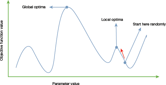FIGURE 10.9 Global and Local Optima
10. Traditional calculus-based mathematical techniques (like gradient-based methods) start at a random point and move in the direction of the gradient until the top of the hill is reached. This technique is efficient and works very well for functions having a single-peak. For example, the cost function in linear regression can easily be solved using gradient-based methods. However, in most real-world problems, there are many peaks and valleys. These problems cannot be solved using the traditional methods as they end-up being stuck at the local optima (refer to Fig. 10.9).

10.2.2 Limitations of Genetic Algorithms

1. Genetic algorithms are not suited for all problems such as those that are either very simple or those for which derivative information is available.
2. The algorithm is computationally expensive for some problems as fitness value is calculated repeatedly.
3. There is no guarantee on the optimality or the quality of the solution.
4. Genetic algorithms may not find the optimal solution if not implemented properly.

10.2.3 Basic Terminology

To understand genetic algorithms, let us familiarize with some basic terminology that will be frequently used.

1. Population: It is a subset of all the possible solutions to the given problem.
2. Chromosomes: A chromosome is the individual solution to the given problem.
3. Gene: A gene is one element position of a chromosome.
4. Allele: It is the value which a gene takes for a particular chromosome. 
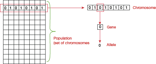
5. Genotype: Genotype is the population (solution) in the computation space that can be represented in a simple and easy-to-understand manner so that it can be easily manipulated using a computing system.
6. Phenotype: Phenotype is the population (solution) in the real-world solution space that can be represented in real world situations (refer Fig. 10.10).
7. Decoding and Encoding: For simple problems, the phenotype and genotype spaces are the same. But for complex, real-world problems, these spaces are different. While decoding is the process of transforming a solution from the genotype to phenotype space, encoding, on the other hand, transforms solution from the phenotype to genotype space. A genetic algorithm must perform decoding at a very fast pace as it has to be done repeatedly while calculating the fitness value.For example, in the 0/1 Knapsack problem, the phenotype space consists of solutions which has the item numbers of the items to be picked. But the genotype space is represented as a binary string of length n (where n is the number of items). A 0 at position x indicates that the x^th item is not picked, whereas a 1 indicates that it was picked. Thus, in this case, genotype space is different from that of the phenotype.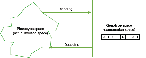FIGURE 10.10 Genotype and Phenotype Space
8. Fitness Function (or Evaluation Function): It is the function which accepts the solution as input and produces the suitability of the solution as the output. That is, the fitness function determines how fit a solution is. This is done by evaluating how close a given solution is to the optimum solution of the desired problem.In some cases, the fitness function and the objective function may be the same but usually they both are different. While the objective function is the function that has to be optimized, fitness function, on the other hand, is the function which guides the optimization.
9. Genetic Operators: Operators which change the genetic composition of the offspring are known as genetic operators. These include crossover, mutation, selection, etc.

10.2.4 Basic Structure

The basic structure of a genetic algorithm can be given as follows.

Step 1: Start with an initial population. The population may either be generated randomly or seeded by using heuristics.

Step 2: Repeat steps 3 and 4 until the specified condition is satisfied.

Step 3: Select parents from this population for producing new offspring. This is done by applying genetic operators like crossover and mutation.

Step 4: Off-springs generated in Step 3 replace the existing individuals in the population.

In this way genetic algorithms mimic the human evolution to some extent.

10.2.5 Genotype Representation

To implement a genetic algorithm (refer Fig. 10.11), we need to first decide how the solutions will be represented. A genetic algorithm can give poor performance if the representation is not correct or inefficient.

Therefore, choosing a proper representation that accurately defines a mapping between the phenotype and genotype spaces is essential for the success of a genetic algorithm.

In this section, we will discuss commonly used representations for genetic algorithms. These representations are problem specific and a mix of these representations is usually used for better results.

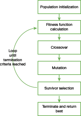
FIGURE 10.11 Steps in a genetic algorithm

Binary Representation

It is one of the simplest and most widely used representation in genetic algorithms. In this representation, the genotype consists of bit strings. Binary representation is best-suited for problems in which the solution space consists of Boolean decision variables—yes or no. For example, in the 0/1 Knapsack problem containing n items, a solution is represented by a binary string of n elements. The value at position is x is 1 if it was picked and 0, otherwise.

For problems that deal with numbers, we can represent the numbers with their binary representation. However, in this encoding, different bits have different significance. Therefore, mutation and crossover operators may have undesired consequences. This can be resolved to some extent by using gray coding.

Real Valued Representation

Real-valued representation is used for representing problems in which genes must have continuous rather than discrete values.

Integer Representation

In some problems, the value of genes cannot be restricted to ‘yes’ or ‘no’, ‘0’ or ‘1’. For discrete valued genes, that can have multiple integer values, integer representation is a preferred choice. For example, four directions—north, south, east and west can be encoded as {0, 1, 2, 3}.

Permutation Representation

Permutation representation is best-suited for problems in which the solution is represented by an order of elements. For example, in the travelling salesman problem (TSP), the salesman has to take a tour of all the cities, visit each city exactly once and come back to the city from where he started. This problem is an optimization problem as the total distance to be travelled has to be minimized. The solution to this problem is an ordering or permutation of all the cities. Hence, permutation representation is used for solving such problems.

10.2.6 Population

As discussed, population is a subset of solutions in the current generation. Every individual in population is called chromosome. So, population can be thought of as a set of chromosomes. In biology, we have read that the population must have diversity to support existence. Similarly, in genetic algorithms, diversity of the population should be maintained to avoid premature convergence.

The size of the population should be chosen very carefully by repeatedly using trial and error technique. While a very large population can slow down the execution of genetic algorithm, a smaller population may not have ‘good’ mating pool. Therefore, an optimal population size needs to be decided by trial and error.

10.2.7 Population Initialization

In a genetic algorithm, population can be initialized in two ways.

1. Random initialization populates random solutions in the initial population. This technique helps to get more optimal solutions. The population is usually defined as a two-dimensional array of − size population, size x, chromosome size.
2. Heuristic initialization uses a known heuristic for the problem to populate the initial population. Note that heuristic initialization should not be used for the entire population as it may in the population having similar solutions with least diversity. Therefore, we can just seed the population with a few good solutions and fill up the rest with random solutions.

10.2.8 Population Models

Genetic algorithms widely use two types of population models:

Steady state, also known as incremental GA, produces one or two off-springs in each iteration. These off-springs replace one or two individuals from the population.

Generational genetic algorithms generate ‘n’ off-springs in each iteration. Here, n refers to the size of the population. In this case, the entire population is replaced by the new one after every iteration.

10.2.9 Fitness Function

The fitness function takes a candidate solution to the problem as input and produces a results statement as output. This output describes how ‘fit’ (or how ‘good’) the solution is with respect to the given problem. The fitness function should be fast as it will be repeatedly applied to find the fitness value. Hence, a slow fitness function can adversely affect the performance of a genetic algorithm. A good fitness function must possess the following characteristics.

1. It should be fast to compute.
2. It must quantitatively measure how fit a given solution is.

For some complex problems, it may not be possible to directly apply the fitness function to calculate the fitness value. In such cases, fitness approximation is done.

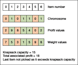
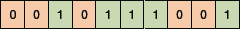
FIGURE 10.12 Calculating Fitness value for a solution of the 0/1 Knapsack problem.

Consider Fig. 10.12 which demonstrates the calculation of fitness value for a solution of the 0/1 Knapsack problem. A simple fitness function is applied which adds the profit values of the items that have been picked. Note that these items have a ‘1’ in their chromosome. We start from the leftmost end and continue to move toward the right until the knapsack is full and cannot take more items. Here, starting from left, we will add values for Item Number 1, 3 and 4, giving a score of 9 + 5 + 4 = 18. We cannot include Item Number 6 because the knapsack capacity will be exceeded. Currently, it is obtained by adding weights of Item Number 1, 3 and 4 which is 5 + 1 + 5 = 11. If we add Item Number 6, then the capacity would be 11 + 8 = 19, which is more than 15 and hence, not possible.

10.2.10 Parent Selection

As the name suggests, parent selection refers to the process of selecting individuals from the population (or parents) which will mate and recombine to generate off-springs for the next generation. Parent selection is a very important task as only ‘good’ parents can produce better and fitter solutions. Therefore, the convergence rate of a genetic algorithm depends on this selection.

While selecting parents, utmost care must be taken to ensure that one extremely fit solution should not take over the entire population in a few generations, as this will diminish diversity in the population and all the solutions produced will be similar to other solutions. One extremely fit solution taking up of the entire population results in a situation known as premature convergence. Clearly, it is an undesirable condition in a genetic algorithm.

The most popularly used technique for selecting parents is the fitness proportionate selection. In this technique, every individual can become a parent with a probability which is proportional to its fitness. This means that fitter individuals have a higher chance of mating and propagating their features to the next generation. Fitness proportionate selection puts selection pressure to fitter individuals in the population, generating better individuals over time.

Consider a circular wheel which is divided into n pies, where n is the number of individuals in the population. Each individual gets a portion of the circle that is in proportion to its fitness value. Given below are two implementations of this technique.

Roulette Wheel Selection

From Fig. 10.13, we see that chromosome A gets a bigger portion of the circle, since it has the highest fitness score. Similarly, other chromosomes have a portion proportional to their fitness score.

In a roulette wheel selection, we have a fixed point on the wheel circumference. When the wheel is rotated, the region of the wheel which comes in front of the fixed point is chosen as the parent. To find the second parent, the same process is repeated.

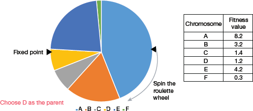
FIGURE 10.13 Roulette Wheel Selection

Since fitter individual has a larger portion of pie on the wheel, it also has a higher chance of coming in front of the fixed point when the wheel is rotated. This clearly indicates that the probability of choosing an individual is directly proportional to its fitness value.

Stochastic Universal Sampling (SUS)

SUS is similar to Roulette wheel selection, but instead of having just one fixed point, the technique has more than one fixed point as shown in Fig. 10.14. Therefore, the parents are selected in a single spin of the wheel. Another advantage of SUS is that it increases the probability of selecting the highly fit individuals at least once (refer Fig. 10.15).

 

Fitness proportionate selection methods do not work for cases where the fitness value is negative.

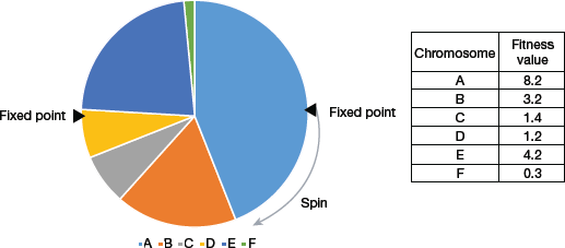
FIGURE 10.14 Stochastic Universal Sampling

FIGURE 10.15

Tournament Selection

In K-Way tournament selection, K individuals are randomly selected from the population and then the best out of K individuals is selected to become a parent (as illustrated in Fig. 10.16). The same process is repeated for selecting the other parent. The main reason for wide acceptability of Tournament Selection is that it can even work with negative fitness values.

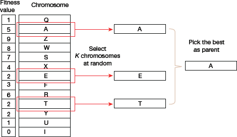
FIGURE 10.16 Tournament Selection

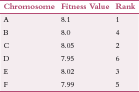
Rank Selection

Rank selection is used when individuals in the population have very close fitness values. In such a situation, if fitness proportionate selection is used, then each individual shares an equal portion of the pie as shown in Fig. 10.17. This indicates that irrespective of one’s fitness value, every individual has nearly the same probability of being chosen to become a parent. Clearly, in this process, there is a reduced focus on selecting fitter individuals, thereby making the genetic algorithm make poor parent selections and thus gives disappointing results.

FIGURE 10.17 Rank Selection

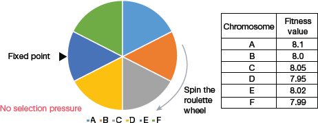
In such a situation, a better technique is rank the individuals in the population based on their fitness values. Therefore, the selection of the parents depends on the rank of each individual and not its fitness score. Higher the rank, higher is the probability of being chosen as a parent. Rank selection can work with negative fitness values as well.

Random Selection

In this strategy, parents are selected randomly from the existing population. There is no pressure to select fitter individuals. Because of this randomness, this technique is rarely used.

10.2.11 Crossover

The crossover operator is analogous to reproduction and biological crossover. In this technique, more than one parent is selected and one or more off-springs are produced using the genetic material of the parents. Given below are some crossover operators which are generic in nature. However, designer of the algorithm may even implement a problem-specific operator.

1. One Point Crossover: In this technique (illustrated in Fig. 10.18), a random crossover point is selected. Then, new off-springs are generated by swapping the tails of its two parents. 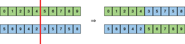FIGURE 10.18 One Point Crossover
2. Multi-point Crossover: It is a generalization of the one-point crossover as it produces new off-springs by swapping alternating segments. Note that in Fig. 10.19, we have two (not one) crossover points. 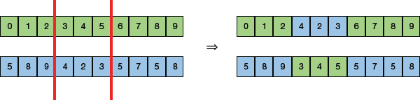FIGURE 10.19 Multi-point Crossover
3. Uniform Crossover: Instead of dividing the chromosome into segments, uniform crossover treats each gene separately (as shown in Fig. 10.20). Each gene may or may not be included in the offspring. To determine whether to include that genet or not, a coin is flipped for each chromosome. We can also add a bias in this technique to bias the coin to one parent. This will help the offspring to get more genetic material that particular parent. 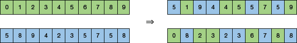FIGURE 10.20 Uniform Crossover
4. Whole Arithmetic Recombination: For integer representations, we take the weighted average of the two parents by using the formula,
   • Child1 = α.x + (1−α).yChild2 = α.x + (1−α).y
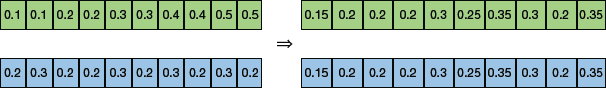   So, diverse offspring can be obtained by varying they value of α . If α = 0.5, then both the children will be identical as shown in Fig. 10.21.FIGURE 10.21 Whole Arithmetic Recombination
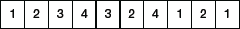
5. Davis’ Order Crossover (OX1): OX1 is used for permutation-based crossovers. Follow the steps given below to apply this operator.

Step 1: Create two random crossover points in Parent 1.

Step 2: Copy the segment between the two crossover points from the first parent.

Step 3: Starting from the second crossover point in the second parent, copy the remaining unused numbers from the second parent to the child.

Repeat the steps while wrapping around the list.

Step 4: If you desire a second child from the two parents, flip Parent 1 and Parent 2 and go back to Step 1.

Example: Consider the solution given in Fig. 10.22. We have two parents.

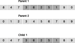
FIGURE 10.22 Davis’ Order Crossover

The child is produced by copying elements 3, 6, 2, 5, 1 from the first parent (according to Step 2).

Then, we copy elements from parent 2 that have not been used so far. Starting on the right side of the second crossover point, grab alleles from parent 2 and insert them in Child 1 at the right edge of the second crossover point. Since 8 is in that position in Parent 2, it is inserted into Child 1 first. Similarly, element 9 and 0 from Parent 2 are copied in Child 1 at the right of second crossover point (while wrapping around the list).

Since elements 1 and 2 from parent 2 are already in child, we will not copy them again.

Copy elements 4 and 7 from Parent 1 to complete the chromosome.

10.2.12 Mutation

Mutation is the process in which a new solution is obtained by introducing a small random tweak in the chromosome. Mutation plays an important role in genetic algorithms as it maintains as well as introduces diversity in the genetic population. Mutation performs ‘exploration’ of the search space and is very essential for a genetic algorithm to converge successfully.

In this section, we will discuss some widely used mutation operators. A genetic algorithm designer can use one of operators or a combination of two or more operators or use a problem-specific mutation operator.

1. Bit Flip Mutation: In this technique (illustrated in Fig. 10.23), one or more bits are selected randomly and flipped. However, it is applied on binary encoded genetic algorithms. FIGURE 10.23 Bit Flip Mutation
2. Random Resetting: It is an extension of the bit flip technique. Random setting operator is used for genetic algorithms that use integer representation. It selects a random value from the set of permissible values and assigns it to a gene that is again chosen randomly.
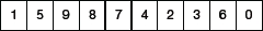
3. Swap Mutation: According to this approach (demonstrated in Fig. 10.24), two positions on the chromosome are selected randomly and their values are swapped (interchanged). This operator is commonly used in permutation-based encodings. FIGURE 10.24 Swap Mutation
4. Scramble Mutation: It is a popular technique used with genetic algorithms that use permutation representations. As the name suggests, scramble mutation selects a subset of genes from the chromosome and then randomly scrambles (or shuffles) their values as shown in Fig. 10.25. FIGURE 10.25 Scramble Mutation
5. Inversion Mutation: As in scramble mutation (refer Fig. 10.26), inversion mutation also choses a subset of genes but instead of shuffling the subset, the string in the entire subset is inverted. FIGURE 10.26 Inversion Mutation

Survivor Selection

The survivor selection policy is used to determine which individuals will be a part of the next generation and which will be discarded. This is an important step to ensure that the fitter individuals are passed on to the next generation. We also need to ensure that diversity in the population should be maintained in every generation.

Some genetic algorithms use the strategy of elitism, which ensures that the fittest member of the current population is always propagated to the next generation. Therefore, under no circumstance can the fittest member of the current population be replaced. Though it is the simplest way to kick random members out of the population, this approach frequently suffers from convergence issues. Therefore, policies discussed below are widely used.

Age-Based Selection

Age-based selection does not consider fitness value for selection. It allows each individual in the population to reproduce for a finite generation. After that, irrespective of how good it is, it is kicked out of the population.

For example, in Fig. 10.27, we see that age is a number that specifies for how many generations the individual has been in the population. The oldest members of the population, P4 and P7 are kicked out of the population and the ages of the other members are incremented by one.

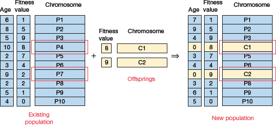
FIGURE 10.27 Age-Based Selection

Fitness-Based Selection

In this selection strategy, the children replace the least fit individuals in the population. The least fit individuals can be selected using any selection policies (like tournament selection, fitness proportionate selection, etc.).

For example, in Fig. 10.28, we see that the least fit individuals P1 and P10 of the population are replaced by the children. Note that P1 and P9 also have the same fitness value, so even they could have been removed. The decision of which individual to remove from the population is arbitrary.

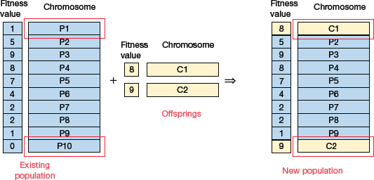
FIGURE 10.28 Fitness-Based Selection

10.2.13 Termination Condition

The termination condition of a genetic algorithm determines when the execution of the algorithm will halt. It has been observed that a genetic algorithm initially works very fast and gives good better solutions in subsequent iterations. But once the saturation point is reached, the improvements in solutions become almost negligible. At such a point, it is better to terminate the algorithm. The termination condition must give a solution that is close to the optimal. The algorithm can terminate under the following conditions:

1. When there is no improvement for X iterations in the population.
2. When the absolute number of generations has been reached.
3. When a certain pre-defined value of the objective function value has been reached.

To implement termination condition in a genetic algorithm, we can maintain a counter (with initial value = 0), to track the generations for which there has been no improvement in the population. When the generated off-spring is not better than the individuals in the population, the counter is incremented.

If the fitness value of any of the off-springs is better than other individuals in the population, then the counter is again reset to zero. The algorithm terminates when the value of the counter becomes equal to a predetermined value. Like other parameters, the termination condition of a genetic algorithm is specific to the problem at hand. And the designer of the genetic algorithm should try various options to see what best-suits that particular problem.

10.2.14 Application Areas

Genetic algorithms are widely used in a variety of application areas as given below.

1. Optimization: Genetic algorithms are widely used in optimization problems. The goal here is to either maximize or minimize the value of a given objective function as per the specified constraints. Genetic algorithms can also be used for multimodal optimization to find multiple optimum solutions. Travelling salesman problem (TSP) can also solve optimally using genetic algorithms.
2. Economics: Economic models (like the cobweb model, game theory equilibrium resolution, asset pricing, etc.) are characterized using genetic algorithms.
3. Neural Networks: Genetic algorithms are used to train neural networks, particularly recurrent neural networks.
4. Parallelization: Genetic algorithms can perform parallel computations. Therefore, these algorithms can effectively solve certain complex problems.
5. Image Processing: Digital image processing (DIP) and dense pixel matching can be easily performed using genetic algorithms.
6. Scheduling applications: Scheduling problems, particularly the time tabling problem, can easily be solved by genetic algorithms.
7. Machine Learning: Genetic algorithms is an important concept used in machine learning algorithms.
8. Robot Trajectory Generation: Genetic algorithms can be used to plan the path which will be taken by a robot arm while moving from one point to another.
9. Parametric Design of Aircraft: Better aircraft designs can be obtained by applying genetic algorithms while varying certain important parameters.
10. DNA Analysis: Genetic algorithms when applied on spectrometric data about the sample, can be used to determine the structure of DNA.