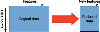
Transfer learning is the reuse of a pre-trained model on a new problem (as shown in Fig. 10.34). So, a machine exploits the knowledge gained from a previous task to improve generalization about another. For example, a classifier that is trained to predict whether an image contains food or not can also be used to recognize drinks with the help of knowledge it gained during the training process.
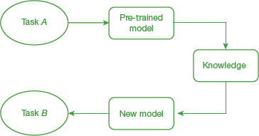
FIGURE 10.34 Transfer Learning
It is currently being used in deep learning in which deep neural networks are trained with very limited data. Since most of the real-world applications do not have millions of labelled data points to train complex models, transfer learning is an important concept.
In transfer learning, we transfer the weights that a network has learned at ‘task A’ to a new ‘task B.’ While task A has a lot of labelled training data available, task B on the other hand, lacks volumes of data. In such a scenario, transfer learning starts the learning process with patterns learned from solving a related task rather than starting from the scratch.
Though transfer learning is not a machine learning technique, it is popularly used in combination with neural networks that require huge amounts of data and computational power. Applications like computer vision and natural language processing extensively use this technique.
10.4.1 How Transfer Learning Works?
In a computer vision application, neural networks detect edges in the earlier layers, shapes in the middle layer and some task-specific features in the later layers. Similarly, in transfer learning, we use the early and middle layers of the model and retrain the latter layers. It helps to take advantage of labelled data of the task it was initially trained on and then transfer as much knowledge as possible from the previous task.
10.4.2 When to Use Transfer Learning
Some guidelines which dictate when transfer learning might be used are as follows and summarized in Fig. 10.35:
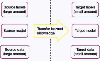
FIGURE 10.35 When to Use Transfer Learning
- When there is very limited labelled training data available to train the neural network from scratch.
- When there is a neural network that has already been trained on a similar task with massive amounts of data.
- When the two tasks have the same input.
- If the existing model was trained using an open-source library (like TensorFlow), you can simply restore some layers and retrain others for the task at hand.
Transfer learning is an optimization, a shortcut to save time and get better performance. Lisa Torrey and Jude Shavlik described three possible benefits to look for when using transfer learning:
- Higher start: The initial skill on the source model before even the model was refined, is higher than it otherwise would be (refer Fig. 10.36).
- Higher slope: The rate of improvement of skill during training of the source model is steeper than it otherwise would be.
- Higher asymptote: The converged skill of the trained model is better than it otherwise would be.
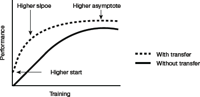
FIGURE 10.36 Graph depicting merits of Transfer Learning
However, the choice of source data or source model is an open problem and may require domain expertise and/or Three ways in which transfer might improve learning intuition developed via experience.
Note that transfer learning only works in the following situations:
- If the features learned from the first task are general so that they can be useful for another related task.
- Input of the model needs to have the same size as it was initially trained with. In case this condition is not satisfied, then resize the input to the needed size.
You can visit pretrained. ml which offers a list of sortable and searchable compilation of pretrained deep learning models with demos and code.
10.4.3 Approaches to Transfer Learning
Training a Model to Reuse It
To solve a task A having limited data to train a deep neural network, find a related task B with an abundance of data. Train the deep neural network on task B and use the same model to solve task A. Whether to use the entire model or just few layers of the model will depend on the problem at hand.
If the input for both the tasks is same, then re-use the model, else make some changes in the task-specific layers of the model before using it.
Using a Pre-Trained Model
Use a pre-trained model but do some research to choose the best one from all available options. Again, whether to reuse the entire model or retrain few task-specific layers depends on the problem to solve. For example, Keras provides numerous pre-trained models that can be used for transfer learning, prediction, feature extraction and fine-tuning. This type of transfer learning is most commonly used throughout deep learning.
Some popular pre-trained machine learning models include the Inception-v3 model, which was trained for the ImageNet to classify images into 1,000 classes like ‘zebra,’ ‘Dalmatian’ and ‘dishwasher.’
Microsoft also offers some pre-trained models that can be used with both R and Python. Developers just have to incorporate the MicrosoftML R and the Microsoftml Python package. Other commonly used models are ResNet and AlexNet.
The more you want to inherit features from a pre-trained model, the more you have to freeze layers.
Feature Extraction
Use deep learning techniques to discover the best representation of the problem. In other words, identify the most important features. This approach is therefore, known as representation learning, and often gives much better performance than hand-designed representation.
Pre-trained model of ImageNet cannot be used with biomedical images because ImageNet does not contain images belonging to the biomedical field.
The learned representation can then be used to solve other problems. But to solve other problems, only first few layers are reused as they are the ones that identify the most useful features of the problem. Latter layers are retrained as they are task-specific. Feature extraction is extensively used in computer vision as it reduces the size of the dataset (refer Fig. 10.37). This, in turn, decreases computation time and enhances the performance of the algorithm.
10.4.4 Traditional Machine Learning vs Transfer Learning
Deep learning experts introduced transfer learning to overcome the limitations of traditional machine learning models. Refer Table 10.6 and Figure 10.38 to see a comparison between Traditional Machine Learning and Transfer Learning.
TABLE 10.6 Differences between traditional machine learning and transfer learning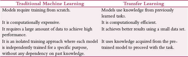
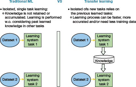
FIGURE 10.38 Traditional Machine Learning vs Transfer Learning
10.4.5 Classical Transfer Learning Strategies
Based on the domain of the application, the problem to solve and the availability of data, we may choose different transfer learning strategies. However, before deciding on the strategy, it is important to have answers for the following questions to improve performance of the target task:
- Which part of the knowledge can be transferred from the source to the targets?
- When to transfer knowledge and when not to?
- How to transfer the knowledge gained from the source model?
Traditionally, there are three types of transfer learning strategies that can be chosen based upon the domain of the task and the amount of labelled/unlabelled data available.
Inductive Transfer Learning
This requires the source and target domains to be the same even if the specific tasks on which the model is working on are different (refer Fig. 10.39).
The algorithms try their best to use knowledge from the pre-trained source model and apply them to improve the target task. Since the source model has the expertise on the features of the domain, it is better to start with it than to start from scratch.
Inductive transfer learning is further divided into two groups—multi-task learning and self-taught learning. While task learning is applicable when the source domain contains labelled data, the latter is used when labelled data is not available.
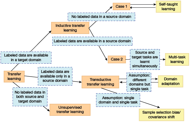
FIGURE 10.39 Inductive Transfer Learning
Transductive Transfer Learning
This type of learning is used when the domains of the source and target tasks are not exactly the same but are interrelated. In this scenario, the source domain has a lot of labelled data but the target domain has only unlabelled data. So, this learning can be used to derive similarities between the source and target tasks.
Unsupervised Transfer Learning
Though this is similar to inductive transfer learning, the algorithms in this approach focus on unsupervised tasks and work on unlabelled datasets both in the source and target tasks.
Transfer learning strategies can also be categorized based on similarity of the domain. This type of division is independent of the type of data samples present for training.
Homogeneous Transfer Learning
As the name suggests, this approach is used when the domains are of the same feature space. There exists only a slight difference in marginal distributions in the domains which can be catered by correcting the sample selection bias or covariate shift.
Instance Transfer
It is done when there is a large amount of labelled data in the source domain, a limited number in the target domain and marginal distributions in both the domains and feature spaces.
For example, imagine that you have to build a model to diagnose cancer in a specific region where there are mostly elderly people. But you have limited target-domain instances. The relevant data are available from another region where the majority comprises young people. In this scenario, directly transferring all the data from another region may not be a viable solution due to the existence of marginal distribution and the fact that elderly have a higher risk of cancer than younger people.
So, here, the marginal distributions are adapted by reassigning weights to the source domain instances in the loss function.
Parameter Transfer
In this technique, it is believed that a well-trained model on the source domain has learned a well-defined structure, and if two tasks are related, this structure can be transferred to the target model. Parameter transfer learning technique transfers the knowledge at the model/parameter level. Knowledge is transferred through shared parameters of the source and target domain learner models. Generally, there are two ways to share the weights-soft weight sharing and hard weight sharing. In soft weight sharing, the model is expected to be close to the already learned features and is penalized if its weights deviate significantly from a given set of weights. In hard weight sharing, the exact weights among different models are shared.
Feature-Representation Transfer
As implicit from the name, this approach transforms the original features to create a new feature representation. This technique can further be categorized as asymmetric and symmetric feature-based transfer learning.
- Asymmetric approaches transform the source features to match the target ones. Therefore, features from the source domain are transformed to make them fit into the target feature space. However, there can be some information loss in this process due to the marginal difference in the feature distribution.
- Symmetric approaches identify a common feature space and then transform both the source and the target features into this new feature representation.
Relational-Knowledge Transfer
This technique focuses on learning the relations between the source and a target domain to extract past knowledge so that it can be used in the current context. Logical relationship or rules learned in the source domain are then transferred to the target domain.
For example, if we learn the relationship between different elements of the speech in a male voice, it can be then used to analyse the sentence in another voice.
Heterogeneous Transfer Learning
In transfer learning, representations from a previous network are derived to extract meaningful features from new samples for an inter-related task. Though this technique seems simple and straightforward, its applicability is not a trivial task due to the following reasons.
- There may exist a difference between the source and the target domain and feature spaces.
- Limited availability of labelled data in the source domain with the same feature space as the target domain.
In such a scenario, heterogeneous transfer learning methods are preferred. This learning strategy is, therefore, applied in cross-domain tasks like cross-language text categorization, text-to-image classification and many others.
10.4.6 Transfer Learning for Deep Learning
Transfer learning is popularly used for applications like NLP and image recognition. There are several pre-trained models that achieve state-of-the-art performance in this field.
Off-The-Shelf Pre-Trained Models as Feature Extractors
We know that deep learning systems comprises multiple layers and each layer learns different features. Initial layers extract higher-level features that narrow down to fine-grained features as we go deeper into the network. These layers are finally connected to the last layer that gives the final output. This opens the scope of using popular pre-trained networks (such as Oxford VGG Model, Google Inception Model, Microsoft ResNet Model) without its final layer to extract a fixed feature for other tasks.
Transfer Learning with Pre-Trained Deep Learning Models as Feature Extractors
In this technique, the pre-trained model’s weighted layers are just used to extract features. The model’s weights are not updated during training with new data for the new task. Since the pre-trained models are trained on a large and general enough dataset, it effectively serves as a generic model of the visual world.
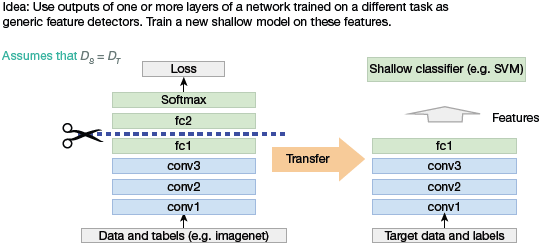
FIGURE 10.40 Transfer learning with Pre-trained deep learning models as feature extractors
Fine Tuning Off-The-Shelf Pre-Trained Models
In this technique, we do not just directly depend on the features extracted from the pre-trained models and replace the final layer. Rather, we selectively retrain some of the previous layers.
Deep neural networks have a layered architecture and have many tunable hyperparameters. While the initial layers capture generic features, the later ones focus on the explicit task at hand. Thus, the higher-order feature representations in the base model must be fine-tuned to make them more relevant for the specific task. We can re-train some layers of the model and keep others frozen in training.
An example is depicted in Fig. 10.41 on an object detection task, where initial lower layers of the network learn very generic features and the higher layers learn very task-specific features.
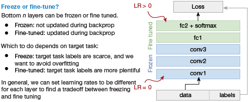
FIGURE 10.41 Freeze vs Fine-tune in Transfer Learning for Deep Learning
Freezing and Fine-Tuning Layers
To increase the model’s performance, we often re-train (or ‘fine-tune’) the weights of the top layers of the pre-trained model and train the newly added classifier. Fine tuning a small number of top layers that are generic rather than the entire model, therefore, it updates the weights for a specific learning and allows the model to apply past knowledge in the target domain and re-learn some things again.
Freezing initial layers to reuse the basic knowledge derived from the past training and fine-tuning higher layers to adapt specialized features to work with the new dataset offers an efficient solution.
10.4.7 Steps in Transfer Learning
Transfer learning can be performed in just a few steps that are illustrated in Fig. 10.42.
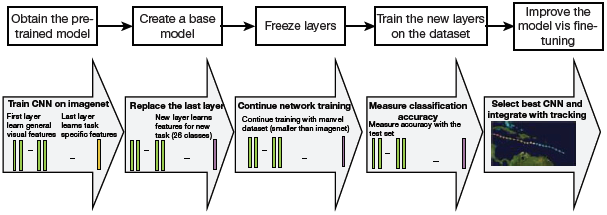
FIGURE 10.42 Transfer Learning process
Step 1: Obtain pre-trained model. The model is kept as the base of our training. Its selection entirely depends on the task at hand. Transfer learning that the knowledge of the pre-trained source model must be directly related and compatible with the target task domain. Few examples of pre-trained models are,
For computer vision: VGG-16, VGG-19, Inception V3, XCeption, ResNet-50
For NLP tasks: Word2Vec, GloVe, FastText
Step 2. Create a base model. The base model is one of the architectures (such as ResNet or Xception) which is in close relation to our task. We can either download the network weights to save time or use the network architecture to train our model from scratch. If the base model has more neurons in the final output layer than required, then we need to remove the final output layer and change it accordingly.
Step 3: Freeze layers. Freeze the starting layers from the pre-trained model to save time in making the model learn the basic features. If we do not freeze the initial layers, the learning already been done will be lost. The process will then be equivalent to training the model from scratch, thereby losing time and other resources.
Step 4: Add new trainable layers. From the pre-trained model, we only use knowledge of feature extraction layers.
Rest of the layers that would perform the specialized tasks needs to be added in the model. These are generally the final output layers.
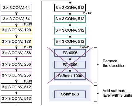
FIGURE 10.43 Fine Tuning the model
Step 5: Train the new layers. The pre-trained model’s final output may be different from that of our new model. For example, if a pre-trained model was trained on the ImageNet dataset to generate 1000 classes and the new task at hand expects the output to be having just two classes, then we have to train the model with a new output layer in place.
Step 6: Fine-tune your model. In this step, we unfreeze some layers of the base model and train the entire model again on the whole dataset at a very low learning rate. This improves performance of the model on the new dataset while preventing overfitting issues (refer Fig. 10.43).
10.4.8 Types of Deep Transfer Learning
Domain Adaptation
It is done when the source and target domains have different feature spaces and distributions. So, domain adaptation technique adapts (or alter) one or more source domains to transfer information to improve the performance of a target learner. The adaptation of source domain is purposely done bring the distribution of the source closer to that of the target.
Domain Confusion
In a neural network, different layers identify different features. For best results, the source and target domains should be as similar as possible. The domain confusion technique creates confusion at the source domain to confuse the high-level classification layers of a neural network. The confusion is created by matching the distributions of the target and source domains to ensure that samples are indistinguishable to the classifier.
While using domain confusion, we need to minimize the classification loss for the source samples, and the domain confusion loss for all samples.
Multi-Task Learning
In this approach (refer Fig. 10.44), several tasks from the same domain are learned simultaneously without distinction between the source and targets. This helps to transfer knowledge from each scenario of the same domain. The shared knowledge helps the learner to optimize the learning (or performance) across all of the n tasks.
Multi-task Learning in Deep Transfer Learning
One-Shot Learning
In this learning, the classification task is given one or a few examples to learn from. After learning, the classifier then classifies many new examples in the future. For example, a face recognition algorithm learns a person’s face that must be classified correctly with different facial expressions, lighting conditions, accessories and hairstyles. This model is fed with one or a few template photos as input.
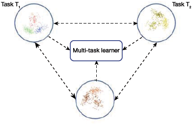
FIGURE 10.44 Multi-Task Learning
Zero-Shot Learning
In this learning technique, transfer learning is done with zero instances of a class. This learning does not depend on labelled data samples. But it does require additional data during the training phase to understand the unseen data.
Zero-shot learning focuses on the traditional input variable, x, the traditional output variable, y, and the task-specific random variable. It is extensively used in applications like machine translation, where we may not have labels in the target language.
10.4.9 Applications of Transfer Learning
- Learning from simulations: Transfer learning is used when traditional machine learning applications that rely on hardware for interaction makes data gathering and model training an expensive and time-consuming or simply too dangerous affair.In such a scenario, simulation is the preferred tool. Transfer learning is done by applying the knowledge gained by simulation process to the real world. Though the feature spaces between source and target domain are the same (both generally rely on pixels), the marginal probability distributions are different, as objects in the simulation and the source look different. Even the conditional probability distributions between simulation and real world might be different as the simulation is not able to fully replicate all reactions in the real world. Udacity has open-sourced the simulator it uses for teaching its self-driving car engineer nanodegree.Learning from simulations has the following benefits:
- Data gathering becomes easy as objects can be easily bounded and analysed.
- Fosters training as learning can be parallelized across multiple instances.
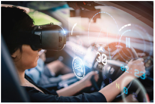 Credit: Have a nice day Photo / ShutterstockFIGURE 10.45 Self-driving car simulator
 - Adapting to new domains: We know that the data where labelled information is easily available and the data that we actually care about are different. Even if the training and the test data look the same, training data may have a bias that is unnoticeable to humans but the model may exploit to overfit on the training data.Domain adaptation is also used to adapt to different text types. For example, if an NLP model is trained, then it will have difficulty coping with more novel text forms such as social media messages.Recently, domain adaptation is also being used in automatic speech recognition (ASR) applications. Such an application may be trained with voice of 500 speakers, but only those people with a similar accent can be benefited. The rest may have trouble being understood.
- Transferring knowledge across languages: Another important application of transfer learning is learning from one language and applying that knowledge to another language. Reliable cross-lingual adaptation methods allow the vast amounts of labelled data in English and apply them to any language, particularly those that are truly low-resource languages.
10.4.10 When Does Transfer Learning Not Work?
Transfer learning should not be used when the weights trained from the source task are different from that of the target task. For example, if the model that was trained to identify tigers cannot be used to identify a sports car. Initializing a model with pre-trained weights that correspond with similar outputs is better than using weights with no correlation with the expected output.
Removing layers from a pre-trained model may cause issues with the architecture of the model. For example, if the first layer is removed, then the model will have a low learning rate as it has to juggle working with low-level features. Moreover, the model may suffer from overfitting issues as removing layers reduces the number of parameters that can be trained. Therefore, using a model with the correct number of layers is vital to the success of a project using transfer learning.
Leave a Reply