
Beam Amplitudes Spot intensity on screen
Left Right as SG
x
is slowly turned off
L R L R Final (SG
x
off)
+ +
+ − no spot
− + no spot
− −
In the language of optics, we can say that the middle two beams, having
26 Introduction to Quantum Physics and Information Processing
opposite phases, destructively interfere so that the corresponding intensity is
zero.
This was an example of interference between just two states. In more com-
plex situations where multiple states exist, each state must be associated with
a phase that is in general complex. It is this phenomenon of interference in
quantum mechanics that calls for description of states with complex ampli-
tudes. In mathematical language, each state is associated with a complex
vector, one that has a magnitude as well as a phase.
The Stern–Gerlach setup we have described in this chapter serves multiple
purposes for us. First, it demonstrates the quantum property of spin of an
electron as a prototypical two-state system that can be used as a qubit. Second,
we can use the setup to prepare a quantum system in a predefined state:
initializing it to |0i or |1i by filtering out one of the outputs. Third, the setup
can be used as a detector to measure the state of the input beam.
Exercise 2.2. Suppose that one of the four beams output from the middle SG
x
were blocked (in Figure 2.9). What would be the intensities of the various
output beams?
Box 2.1: Polarization States of Light
The quantum spin described in this chapter is novel and has no classical
analog. However, the same picture of a 2-dimensional Hilbert space emerges
from considering the polarization states of light. This example is worth con-
sidering, as it will be particularly useful later when we use light for quantum
information processing. The analogy with spin is also complete, with a classi-
cal picture to peg our understanding on.
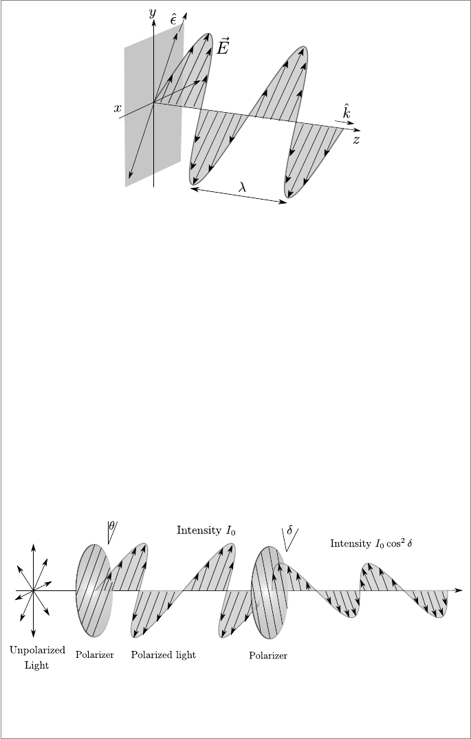
Classically, light is electromagnetic radiation, with oscillating electric and
magnetic fields. The form of the fields comes from solutions to Maxwell’s
equations. It is easier to detect the electric field, so we will describe light by
its electric field vector. The important parameters that describe a monochro-
matic light wave are its wavelength λ and angular frequency (color) ω and the
wave vector
~
k =
2π
λ
ˆ
k giving the direction of propagation. The direction
ˆ
k is
conventionally taken to be ˆz, just as SG
z
is the standard for the spin system.
An important property of the electromagnetic wave in free space is transver-
sality: the electric field vector always lies in a plane perpendicular to
ˆ
k. The
direction of the electric field vector is known as its polarization. This direction
could be constant, as in linearly polarized light, or rotate in the polarization
plane, as in circularly polarized light.
A Simple Quantum System 27
FIGURE 2.10: Linearly polarized light wave.
Let’s first look at linearly polarized light with the
−→
E field oscillating along
a direction we’ll call ˆ (Figure 2.10). It is possible to produce such light by
passing unpolarized light from a monochromatic source through a polaroid
filter. Such a filter has a “pass axis” that allows polarizations parallel to this
axis alone to be transmitted through. The field is described by
−→
E = E
0
ˆ cos(kz −ωt). (2.11)
The intensity of light is given by the magnitude square of the electric field.
If a second polarizer, with its pass-axis at an angle δ to the first, is placed in
the light path, then only the component of the
−→
E field along this angle is
passed through. So the electric field of the transmitted light is E cos δ in a
direction parallel to the new pass axis. The intensity of the light falls by a
factor cos
2
δ (Figure 2.11).
FIGURE 2.11: Effect of a linear polarizer on unpolarized light; subsequent
polarizer allows only a component ∝ cos
2
δ through.
More generally, the electric field could have components oscillating along the
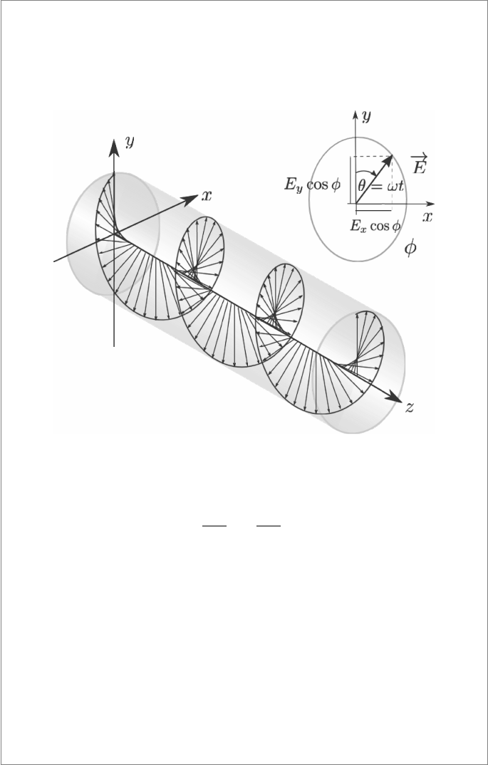
28 Introduction to Quantum Physics and Information Processing
ˆx and the ˆy directions with different amplitudes and even different phases:
−→
E = E
1
ˆxe
i(kz−ωt)
+ E
2
ˆye
i(kz−ωt+φ)
. (2.12)
FIGURE 2.12: Light with elliptic polarization: the electric field vector traces
out an ellipse in the x-y plane
One can define the polarization vector
ˆ =
E
1
|
−→
E |
ˆx +
E
2
|
−→
E |
e
iφ
ˆy.
This is in general elliptical polarization (Figure 2.12). The special case φ = π/2
corresponds to circular polarization while φ = 0 is linear polarization.
It is easy to see that if ˆx-polarized light is incident on a ˆy-polarizer (a polaroid
filter with its pass axis along the ˆy direction), no light passes through. We
can thus define two orthogonal polarization states of light corresponding to
the vertical (ˆy) and horizontal (ˆx) directions. This experiment is analogous
to the Stern–Gerlach-z machine, with up and down ports being analogous to
the vertical and horizontal polarizations. We can thus draw analogy between
the vector space of light polarizations and the spin Hilbert space:
|0i ↔ l
|1i ↔ ↔ .
A Simple Quantum System 29
To create the optical analogue of the states produced by SG
x
filters, we will
need to use polarizers that are rotated by 45
◦
with respect to the earlier ones.
Light produced by these polarizers can be in polarization states
l
and
l
defined by the 45
◦
orthogonal directions:
l
=
1
√
2
(ˆx + ˆy)
l
=
1
√
2
(ˆx − ˆy).
It is easy to see that if
l
light is incident on an ˆx or ˆy polarizer then 50% of
the incident beam passes through. Similarly for
l
.
The analogy of the SG
y
basis is with right and left circular polarization. From
Equation 2.12, we see that light with electric field rotating in the plane of
polarization arises due to a phase difference of π/2 between the x- and y-
components. The complex notation is most suitable for expressing this phase
relationship (using i = e
iπ/2
):
|↑
y
i ↔ =
1
√
2
(ˆx + iˆy) (2.13)
|↓
y
i ↔ =
1
√
2
(ˆx − iˆy) (2.14)
The necessity of complex probability amplitudes becomes clear now, due to
considerations of phase being unavoidable.
Leave a Reply