
We now have an alternate formulation of quantum mechanics, in terms
of density operators instead of state vectors, that is good for open systems
as well. Let’s go through the axioms of quantum mechanics framed in this
language.
5.2.1 States and observables
Postulate 1. Quantum State: The state of a quantum system is described
by a density operator in Hilbert space, i.e., a positive Hermitian operator with
unit trace.
Postulate 2. Observables: An observable A is represented by a Hermitian
operator
ˆ
A on Hilbert space. When measured in a state ρ, the probability of
an outcome a
n
is given by
P(a
n
)
ρ
= Tr(ρ
ˆ
P
n
) (5.24)
where
ˆ
P
n
= |nihn| is the projection on the appropriate eigenspace of
ˆ
A. The
expectation value of the observable is given by
h
ˆ
Ai
ρ
= Tr(ρ
ˆ
A). (5.25)
5.2.2 Generalized measurements
When measurements are made on open systems, we are forced to generalize
our notion (from Section 3.3) of projections on the eigenspaces of the observ-
able being measured. Those are special cases and are called von Neumann or
projective measurements.
Most real measurements are not of this kind. To take a simple but extreme
example: how do we describe the measurement of the position of a photon in
Mixed States, Open Systems, and the Density Operator 89
an experiment where it strikes a screen that emits a phosphorescent flash?
In this case the position may be noted, but the photon has been absorbed
by the screen! Thus we can no longer say the measurement is projective with
the post-measurement state being given by Equation 3.17. In fact the pho-
ton itself is destroyed by measurement. Another assumption of the projective
measurement model is that the measurement is repeatable: successive actions
of the projection operator on the same state give the same result. Most real
measurements are not repeatable. We therefore need to generalize the idea of
measurement.
The main characteristic of any operator representing measurement is that
it must tell us how to calculate the probabilities of outcomes. The projective
measurements considered in Chapter 3 can be expressed in the density opera-
tor formalism as follows. If the outcome is α then the state is transformed by
the projection operator
ˆ
α
= |αihα|:
ρ
Measure
ˆ
A, obtain α
−−−−−−−−−−−−−→
ˆ
α
ρ
ˆ
†
α
. (5.26)
The probability of obtaining the outcome α is given by
P(α) = Tr(
ˆ
α
ρ
ˆ
†
α
) = Tr(
ˆ
†
α
ˆ
α
ρ) = Tr(
ˆ
α
ρ). (5.27)
The last step follows from the orthogonality of projection operators (Equa-
tion 3.21):
ˆ
†
α
ˆ
α
=
ˆ
α
. It is this property that we drop in the case of gener-
alized measurements.
For generalized measurement, we think in terms of a complete set of mea-
surement operators
ˆ
M
m
, each of which corresponds to a different measurement
outcome m. But these operators do not need to be orthogonal like projection
operators.
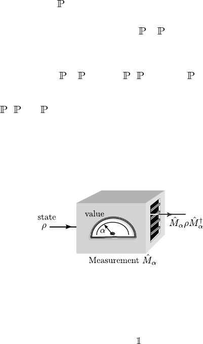
FIGURE 5.4: Generalized measurement.
Postulate 3. Measurement: a measurement process capable of yielding m
possible distinct outcomes can be described by a set of Hermitian measurement
operators
ˆ
M
m
satisfying
P
m
ˆ
M
†
m
ˆ
M
m
= (the completeness relation). The
probability of an outcome m is
P(m) = Tr(
ˆ
M
†
m
ˆ
M
m
ρ) (5.28)
90 Introduction to Quantum Physics and Information Processing
and the state after measurement is given by the density operator
ρ
m
=
ˆ
M
m
ρ
ˆ
M
†
m
Tr(
ˆ
M
†
m
ˆ
M
m
ρ)
. (5.29)
The special case of projective measurements corresponds to
ˆ
M
†
m
ˆ
M
m
≡
|mihm| =
ˆ
m
.
5.2.3 Measurements of the POVM kind
In most applications of measurement, we are not interested in the post-
measurement state of the system, but only in the statistics, or the relative
probabilities of different outcomes, that we can collect by measuring an en-
semble. A special case of the measurement postulate caters to this need, and is
known as the POVM formalism. The set of measurement operators is known
as a positive operator-valued measure
2
or POVM for short. The reason
for this technical-sounding name is not important; we will just describe the
main elements of this formalism here, due to its usefulness and pervasiveness
in literature.
If we consider the set of operators
ˆ
E
m
= M
†
m
M
m
,
X
m
ˆ
E
m
= , (5.30)
then the probability of outcome m on making a measurement on the state ρ
is
P(m) = Tr(
ˆ
E
m
ρ).
It can be easily seen that the operators
ˆ
E
m
are positive, but not necessarily
orthogonal. That is,
ˆ
E
m
ˆ
E
n
6= δ
mn
ˆ
E
m
.
They are called the POVM elements, with the set {
ˆ
E
m
} called the POVM.
For our purposes, the POVM is just a set of positive operators that add up
to unity. Some texts also call these operators as forming a non-orthogonal
partition of unity (as opposed to the orthogonal partition made by projection
operators).
Example 5.2.1. If we consider the projectors
m
= |mihm| as the measure-
ment operators, then POVM elements are
ˆ
E
m
=
†
m
m
=
m
,
the same as the measurements operators themselves. Some texts call these
projection-valued measures or PVMs.
2
The word “measure” becomes relevant only in the case of infinite dimensional Hilbert
spaces.
Mixed States, Open Systems, and the Density Operator 91
Example 5.2.2. One context in which POVM is very useful is in distinguishing
two non-orthogonal states with maximum probability. Consider for example
the states
|ψ
1
i = |0i, |ψ
2
i = |+i =
1
√
2
(|0i + |1i).
The operators |1ih1| and |−ih−| project onto orthogonal subspaces. We can
form a partition of unity by adding a third operator, so that the set
ˆ
E
1
=
2 −
√
2
|1ih1|,
ˆ
E
2
=
2 −
√
2
|−ih−|
ˆ
E
3
= − (
ˆ
E
1
+
ˆ
E
2
).
forms a POVM. Verify that each of the
ˆ
E
i
is positive.
If we measure these operators,
ˆ
E
1
and
ˆ
E
2
giving outcomes yield positive
conclusions: there will be no outcome corresponding to
ˆ
E
1
if the state were
|ψ
1
i, and none corresponding to
ˆ
E
2
if the state were |ψ
2
i. But when the
outcome corresponding to
ˆ
E
3
occurs, then we cannot tell which state we had.
These operators thus give us a way of unambiguously distinguishing the two
states except in the third (inconclusive) case.
The POVM formalism is especially useful when we consider a system in
a mixed state as a subspace of a larger system in a pure state. If we per-
form projective measurements on a larger space, the effect on the subspace
is of POVM measurements (see Box 5.1). This is in fact the motivation for a
theorem due to Neumark, which states that any POVM can be realized as a
projective measurement on an extended Hilbert space.
5.2.4 State evolution
How is the evolution of a system described in terms of density matrices?
The evolution operator U for a closed system must be unitary. So for a closed
system evolving from initial time t
0
= 0 to some final time t, we can write
ρ(t) = U(t)ρ(0)U
†
(t). (5.31)
For a mixed state, ρ =
P
n
p
n
|ψ
n
ihψ
n
|. Assuming that time evolution pre-
serves this linearity, we can extend Equation 5.31:
ρ(t) =
X
n
p
n
U(t)|ψ
n
ihψ
n
|U
†
(t). (5.32)
Now the unitary time-evolution operator is obtained from the energy operator,
or Hamiltonian
ˆ
H for the system:
ˆ
U(t) = exp(−i
ˆ
H(t − t
0
)/~)
Leave a Reply