
Let’s start with 1-bit functions f : {0, 1} 7→ {0, 1}. There are totally
four possible functions, and evaluated on inputs 0 and 1 can give answers
0 or 1. To actually determine which of these our black box is we need to
query it with both inputs, whether classically or otherwise, and we obtain no
Quantum Algorithms 145
advantage using quantum computing. However, as David Deutsch [24] showed
in 1985, it is possible to distinguish the function on the basis of some property,
more efficiently in the quantum case. The particular classification Deutsch’s
algorithm considers is the following: they are either constant (C), i.e., f(0) =
f(1), or balanced (B), i.e., the outputs contain an equal number of 0’s and 1’s
(f(0) = f (1)).
Example 8.1.1. For n > 1, functions need not fall into the classes C or B
alone. For example, consider f
1
and f
2
defined by:
f
1
:
f(00) = 0
f(01) = 1
f(10) = 0
f(11) = 1
, f
2
:
f(00) = 0
f(01) = 1
f(10) = 0
f(11) = 0
Here, f
1
is balanced while f
2
is neither constant nor balanced.
Deutsch’s algorithm
1
is formulated for the following problem. Although it
might seem contrived, it is the first algorithm to demonstrate the principles
of the new paradigm.
The problem: given a black-box (oracle) that implements a 1-bit function
f(x), how will you determine whether the function belongs to class C or to
class B with a minimum number of runs of the black box (or equivalently,
queries to the oracle)?
Classically, it is clear that we have to run the machine twice, with inputs
0 and 1.
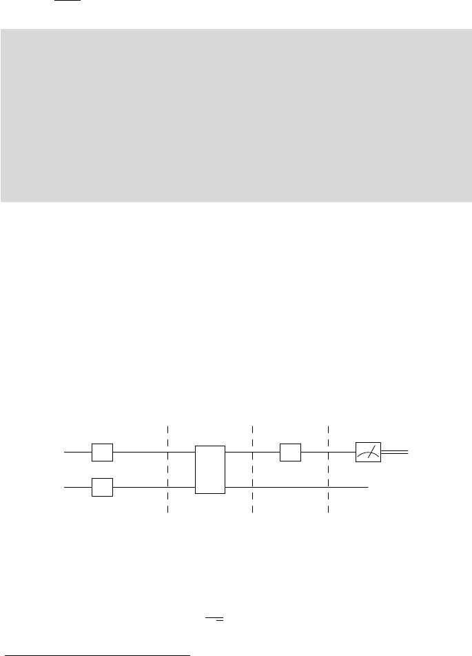
The Deutsch algorithm shows how this problem can be solved in just
one run of the black box. The circuit is shown in Figure 8.3, that we will work
through step by step.
|0i
H
|+i
U
f
H
(
0 7→ C
1 7→ B
|1i
H
|−i
|ψ
0
i |ψ
1
i |ψ
2
i
FIGURE 8.3: The Deutsch algorithm.
Step 1: Supply as input the uniform superposition
H|0i =
1
√
2
(|0i + |1i). (8.1)
1
The presentation given here is not the original one in [24] but an improved version
146 Introduction to Quantum Physics and Information Processing
Step 2: On the bottom register, supply the state H|1i =
1
√
2
(|0i−|1i). This is
the crucial feature that introduces useful interference in the result. The reason
for this will be clear when we evaluate the output of the black box. So the
input state is
|ψ
0
i =
1
√
2
(|0i + |1i) ⊗
1
√
2
(|0i − |1i)
=
1
2
[|00i − |01i + |10i − |11i] (8.2)
Step 3: Run the function evaluator. The output is
|ψ
1
i = U
f
|ψ
0
i
=
1
2
h
|0i|f(0)i − |0i|f (0)i + |1i|f(1)i − |1i|f(1)i
i
=
1
2
|0i
h
|f(0)i − |f (0)i
i
+
1
2
|1i
h
|f(1)i − |f (1)i
i
. (8.3)
Step 4: Measure the top register in the X-basis. That is, change basis by
applying the H gate on the first qubit and then measure it. Just before the
measurement, the output state on both wires is
|ψ
2
i = H
1
|ψ
1
i
=
1
2
√
2
|0i
h
|f(0)i − |f (0)i + |f(1)i − |f(1)i
i
+
1
2
√
2
|1i
h
|f(0)i − |f (0)i − |f(1)i + |f(1)i
i
(8.4)
If the function is C, then f(0) = f(1) and the amplitude for |0i is 1 while
that for |1i is 0. On the other hand, when f is B then f(0) = f(1) and
the amplitude for |1i is 1 while that for |0iis 0. Thus a measurement of
the output gives us the answer to the query with certainty. We have run the
function evaluator only once. The quantum advantage has given us a double
speedup in this case.
The reason why this works is that Step 2 implements the so called “phase
kickback” trick. If the state |−i on the lower register fed into the black box,
then the output acquires a phase that depends on f(x). This phase can effec-
tively be regarded as attached to the state of the upper register.
U
f
|xi ⊗
(|0i − |1i)
√
2
=
1
√
2
|xi
h
|f(x)i − |f (x)i
i
=
(
1
√
2
|xi(|0i + |1i) if f (x) = 0,
1
√
2
|xi(|1i − |0i) if f (x) = 1
= (−1)
f(x)
|xi
1
√
2
[|0i − |1i] . (8.5)
Quantum Algorithms 147
The output is separable, with the lower register unchanged in state |−i, while
the upper register is effectively the input with an f(x)-dependent phase.
With this effect, we can re-analyze the algorithm with the uniform super-
position |xi =
1
√
2
(|0i + |1i) in the input register:
1
√
2
(|0i + |1i)
U
f
−−→
1
√
2
h
(−1)
f(0)
|0i + (−1)
f(1)
|1i
i
(8.6)
H
−→
1
√
2
h
(−1)
f(0)
+ (−1)
f(1)
|0i
+
(−1)
f(0)
− (−1)
f(1)
|1i
i
(8.7)
where it’s obvious that a measurement gives |0i if f(x) is C and |1i if f(x)
is B.
8.1.1 Deutsch–Josza algorithm
The Deutsch algorithm was extended to n-bit functions by Josza and others
in 1992 [26].
The problem: Given an n → 1 function f : {0, 1}
n
7→ {0, 1} that is
guaranteed to be either constant or balanced, find out which it is in a minimum
number of runs.
Classically, we would proceed by querying the oracle with each n-bit
number. If we find an answer that is not equal to the previous one then we
have a balanced function. In worst-case scenario, we might find the same f(x)
until the half the possible inputs, i.e., after querying the function 2
n
/2 times.
The answer to the next query would solve the problem. Thus we need to run
the oracle at worst 2
n−1
+ 1 times: exponential in the number of bits of input.
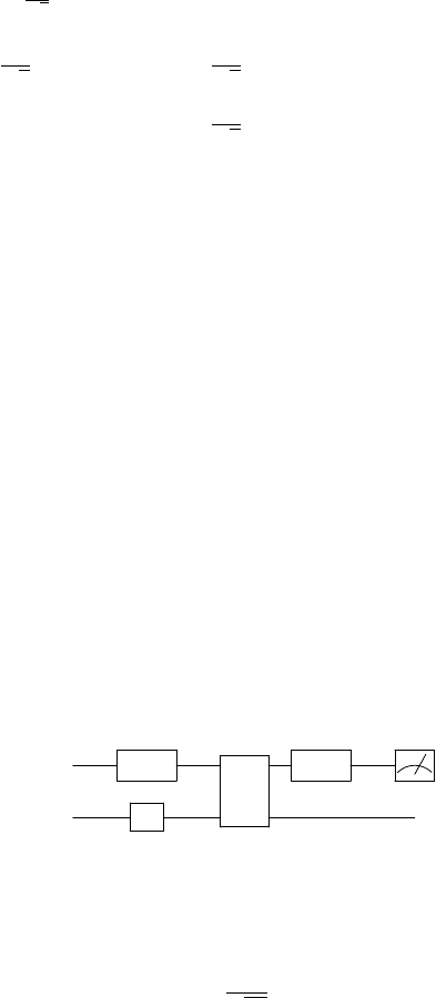
The quantum algorithm achieves the distinction in just one run! This
is a dramatic speedup indeed. The circuit (Figure 8.4) is an n-qubit extension
of that for the Deutsch problem:
|0i
n
/
n
H
⊗n
/
n
U
f
H
⊗n
/
n
|1i
H
FIGURE 8.4: The circuit for the Deutsch–Josza algorithm.
The input to the circuit is the uniform n-qubit superposition
H
⊗n
|0i
n
=
1
√
2
n
2
n
−1
X
x=0
|xi. (8.8)
Leave a Reply