
The quantum Fourier transform (QFT) is simply the DFT operation on the
amplitudes of a quantum state. The DFT matrix is unitary, and can therefore
represent a quantum transformation. We can define the QFT (order N = 2
n
)
of an n-qubit basis state |xi by
ˆ
F
N
|xi =
1
√
N
N−1
X
y=0
ω
xy
N
|yi. (8.37)
Interestingly, as we have seen in Equation 8.26, the QFT transform for n = 2
is just the Hadamard gate.
When applied to a superposition state |ψi =
P
i
C
i
|ii, the QFT performs
a DFT on the coefficients C
i
:
ˆ
F
N
|ψi =
X
i
C
i
U
N
|ii
=
1
√
2
n
X
i
C
i
X
j
ω
ij
N
|ji (8.38)
=
X
j
DFT
N
C
j
|ji. (8.39)
where C denotes the vector of coefficients in the state representation.
An efficient algorithm for evaluating the QFT is inspired by the FFT
algorithm, where we compute the bit-wise breakup of the action of
ˆ
F on its
Quantum Algorithms 159
input. Remember, |yi
n
=
N
n−1
j=0
|y
j
i. Each y
j
takes a value 0 or 1. The QFT
has superpositions of |yi with a phase ω
xy/N
N
, containing the integer product
of x and y. We want to break this up into the constituent bits, the y
j
s. So we
write
xy =
x
0
+ 2x
1
+ ··· + 2
n−1
x
n−1
y
0
+ 2y
1
+ ···2
n−1
y
n−1
. (8.40)
Now any product in this expansion that has a coefficient of 2
n
or higher can
be dropped since it would contribute unity to the phase: ω
2n
N
= 1. So we find
xy
N
=
x
0
2
n
+
x
1
2
n−1
+ ··· +
x
n−1
2
y
0
+
x
0
2
n−1
+
x
1
2
n−2
+ ··· +
x
n−2
2
y
1
.
.
.
+
x
0
2
2
+
x
1
2
y
n−2
+
x
0
2
y
n−1
. (8.41)
Using the binary “point” notation
0.x
1
x
2
x
3
…x
n
=
x
1
2
+
x
2
2
2
+
x
3
2
3
+ …
x
n
2
n
, (8.42)
xy
N
= y
0
(0.x
n−1
x
n−2
···x
0
) + y
1
(0.x
n−2
···x
0
) + ··· + y
n−1
(0.x
0
). (8.43)
Using this to write the QFT in bit-wise expansion, we can associate an expo-
nential factor with each bit of y, the output becomes the following product
state:
ˆ
F
N
|xi =
1
√
2
n
X
y
e
2πixy/N
|y
0
i ⊗ |y
1
i···|y
n−1
i
=
1
√
2
n
X
y
0
=0,1
e
2πiy
0
(0.x
n−1
x
n−2
···x
0
)
|y
0
i
!
⊗
X
y
1
=0,1
e
2πiy
1
(0.x
n−2
···x
0
)
|y
1
i
!
⊗
··· ⊗
X
y
n−1
=0,1
e
2πiy
n−1
(0.x
0
)
|y
n−1
i
=
|0i + e
2πi(0.x
n−1
x
n−2
···x
0
)
|1i
√
2
⊗
|0i + e
2πi(0.x
n−2
···x
0
)
|1i
√
2
⊗
··· ⊗
|0i + e
2πi(0.x
0
)
|1i
√
2
(8.44)
160 Introduction to Quantum Physics and Information Processing
Each term in the product of Equation 8.44 is the state of an output qubit
for the corresponding qubit of the input. This translates into a circuit for
evaluating
ˆ
F
2
n
. The order of occurrence of the terms must be noted: the first
term is the least significant bit, and the last is the most significant bit of the
output.
Example 8.5.1. QFT circuit for n = 2:
|x
1
x
0
i
ˆ
F
−→
|0i + e
2πi(0.x
0
)
|1i
√
2
⊗
|0i + e
2πi(0.x
1
x
0
)
|1i
√
2
This means
|x
1
i −→
|0i + e
2πi(
x
0
2
)
|1i
√
2
= |y
1
i
|x
0
i −→
|0i + e
2πi(
x
1
2
+
x
0
4
)
|1i
√
2
= |y
0
i
Here |y
1
i has an x
0
-dependent phase of e
iπ
for |1i, which can be obtained
by an H acting on |x
0
i. Similarly |y
0
i has a x
1
-dependent phase of e
iπ
and
an x
0
-dependent phase of e
iπ/2
for |1i. The first is obtained by an H on |x
1
i
while the second is the x
0
-controlled action of the gate R
1
=
1 0
0 e
iπ/2
!
:
|x
1
i
H
R
1
|y
0
i
|x
0
i
•
H
|y
1
i
Note that the output is to be read in reverse order!
Exercise 8.4. Work out the circuit for the QFT for n = 3.
|x
n−1
i
H
R
n−1
R
n−2
. . .
R
1
|y
0
i
|x
n−2
i
•
H
R
n−2
R
n−3
. . .
|y
1
i
.
.
.
.
.
.
.
.
.
|x
1
i
• •
H
R
1
|y
n−2
i
|x
0
i
• • •
H
|y
n−1
i
FIGURE 8.10: Circuit for the quantum Fourier transform
ˆ
F
2
n
, on n qubits.
You should now be able to work out that Figure 8.10 is an efficient quantum
circuit for the QFT on n qubits.. We require controlled phase gates, with phase
Quantum Algorithms 161
matrices like
R
d
=
1 0
0 e
iπ/2
d
!
, (8.45)
where d can be interpreted as the distance from the control bit. Notice that
the output bits are in reverse order. One can either agree to read the output
in reverse order or to perform a swap at the end.
The efficiency of this circuit is related to the number of basic gate oper-
ations required per input bit. We can easily see that this is n H-gates and
n(n − 1)/2 C-R-gates for n bits, which is O(n
2
). This is exponentially faster
than the classical FFT which takes O(n2
n
). Hurray for quantum algorithms!
But before we exult too much, observe that the output of the quantum
Fourier transform is a superposition of basis states whose phases represent the
Fourier transform of the corresponding input bit. A measurement at the end of
the above circuit gives us no information whatsoever about the Fourier trans-
form of the input! So we cannot use this circuit as a super-efficient Fourier
transform computer! Instead, we have to incorporate it in procedures that re-
quire FT-dependent phases. And Peter Shor did just that in his path-breaking
algorithm for prime factorization.
8.5.1 Period-finding using QFT
Preliminary to the Shor algorithm, let’s focus on one that lends itself
naturally to the QFT: computing the period r of a periodic n-bit function
f : {0, 1}
n
7→ {0, 1}
n
such that f(x + r) = f(x), r ∈ [0, 2
n
− 1]. (8.46)
We will take 2
n
= N in what follows. The function could repeat more than
once in the interval [0, N − 1], so we have
f(x + kr) = f (x), kr < N.
We assume we are presented with a black box (oracle) that evaluates such a
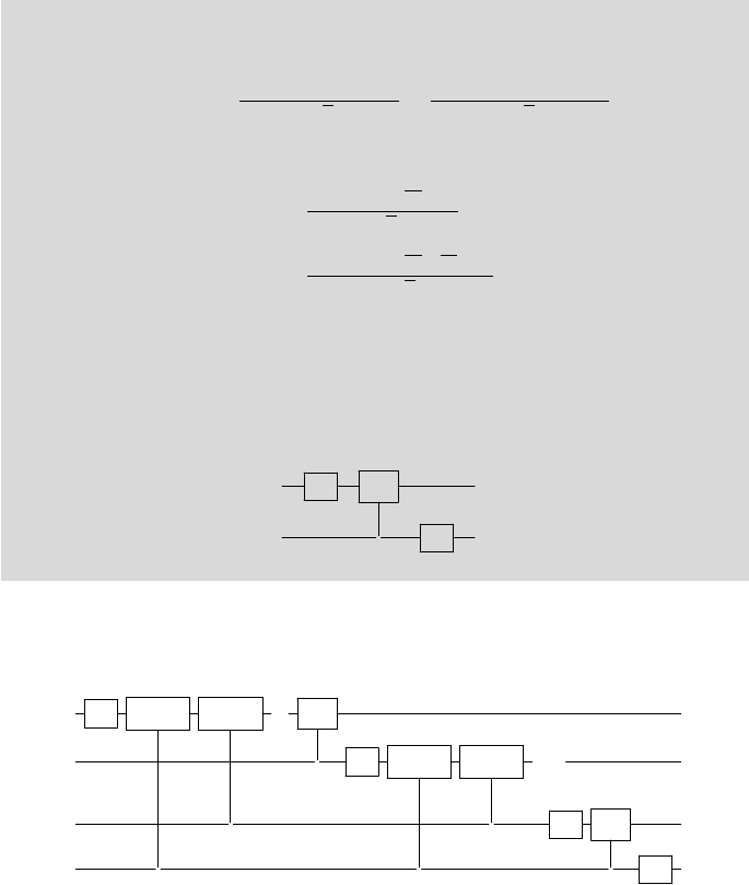
function. The algorithm uses a circuit that is a direct extension of Simon’s
algorithm (Section 8.3), in which we’ll use the full QFT instead of the 1-bit
version (the Hadamard transform) used there. The circuit (Figure 8.11) is
straightforward.
|0i
n
/
n
H
⊗n
U
f
/
n
ˆ
F
N
/
n
|0i
n
/
n
|ψ
0
i |ψ
1
i
FIGURE 8.11: Circuit for quantum period finding.
162 Introduction to Quantum Physics and Information Processing
The input to the U
f
black box is once again
|ψ
0
i =
1
√
N
N−1
X
x=0
|xi
n
⊗ |0i
n
, (8.47)
So the output ought to be
|ψ
1
i =
1
√
N
N−1
X
x=0
|xi ⊗ |f(x)i. (8.48)
We will again assume that we measure the lower register at this point, ob-
taining some number f
0
. Then the top register collapses to a superposition of
only those states |xi for which f(x) = f
0
. All such x’s are of the form x
0
+ kr
for some x
0
< r, and some integer k : kr < N. Suppose the number of periods
within the interval [0, N − 1] is p:
p = [N/r] , (8.49)
where the square bracket notation stands for the ceiling function (greatest
integer less than the argument). The state of the computer is then a superpo-
sition of p terms of the form
|ψ
1
i =
1
√
p
p−1
X
k=0
|x
0
+ kri ⊗ |f
0
i. (8.50)
Now subjecting the top register to a QFT, we get
ˆ
F
N
1
√
p
p−1
X
k=0
|x
0
+ kri
!
=
N−1
X
y=0
1
√
Np
p−1
X
k=0
e
2πi(x
0
+kr)y/N
!
|yi. (8.51)
This is a superposition of basis states with a probability of occurrence of a
particular y given by the mod-squared of the term in the brackets:
P(y) =
1
Np
p−1
X
k=0
e
2πi(x
0
+kr)/N
2
=
1
Np
p−1
X
k=0
e
2πikry/N
2
(8.52)
So y has an r-dependent probability of occurrence. The crux of this algorithm
is that the most probable value of y gives us enough information about r for
us to compute it. In fact, the claim is that the values of y that are measured
are close to an integer multiple of N/r.
Let’s first see this in the special case when there are exactly integer number
of periods in the interval [0, N − 1], i.e., when
p =
N
r
.
We will compare the probability of y for mp when m is some integer, and
when not:
P(y) =
1
r
1
p
p−1
X
k=0
e
2πiky/p
2
. (8.53)
P(y = mp) =
1
r
, (8.54)
P(y 6= mp) =
1
rp
2
p−1
X
k=0
e
ikθ
2
, where θ = 2π
y
p
, (8.55)
=
1
rp
2
sin
2
(pθ/2)
sin
2
(θ/2)
= 0
since pθ is an integer multiple of 2π
. (8.56)
So the only values of y obtained in this case are integer multiples of N/r.
For a general function, it is highly unlikely that there are exactly integer
numbers of periods in the interval [0, N −1]. Yet, the most probable values of
y turn out to be close to integer multiples of N/r! To see this, let us start by
writing
y = m
N
r
+ δ
m
, (8.57)
where m is an integer and |δ
m
| ≤
1
2
. Let’s substitute this in Equation 8.52:
P(y) =
1
Np
p−1
X
k=0
e
2πikr(mN/r+δ
m
)/N
2
=
1
Np
p−1
X
k=0
e
2πikrδ
m
/N
2
=
1
Np
sin
2
(pθ
m
)
sin
2
θ
m
, where θ
m
=
πr
N
δ
m
. (8.58)
Now since p is nearly N/r, the numerator is nearly sin
2
(πδ
m
). Also, rδ
m
/N
is very small, so the denominator is nearly θ
m
∼ πδ
m
r/N.
Therefore,
P(y) ∼
1
Np
sin
2
(πδ
m
)
(πδ
m
r/N)
2
=
1
r
sin
2
(πδ
m
)
(πδ
m
)
2
. (8.59)
Since δ
m
< 1/2, and
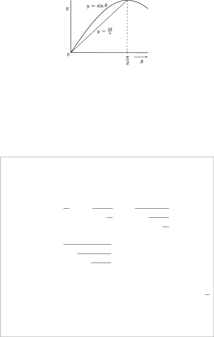
sin θ
θ
≥
2
π
for 0 ≤ θ ≤ π/2, (see Figure 8.12), we have
P(y ∼ m/r) ≥
4
π
2
r
. (8.60)
164 Introduction to Quantum Physics and Information Processing
FIGURE 8.12: Graph comparing sin θ and 2θ/π.
There are r possible such y’s, so the probability of any such y is greater
than 4/π
2
∼ 40%. This result is to be interpreted as saying that when we
rerun the algorithm many times, with high probability we measure y’s that
are integer multiples of N/r. Now from such numbers we can use classical
algorithms to deduce r, most famously the Euclid algorithm for continued
fractions. The period-finding algorithm thus succeeds to a high probability.
Such analyses of the probability of obtaining good results are a common
feature of most known quantum algorithms.
Box 8.3: Finding r Given N/r: Continued Fractions
The output y of a run of the period-finding algorithm is close to an integer
multiple of N/r. Consider the number x = y/N ∼ m/r. We now look at the
continued fraction expansion of x:
x = c
0
+
1
x
1
= c
0
+
1
c
1
+
1
x
2
= c
0
+
1
c
1
+
1
c
2
+
1
x
3
= ··· (8.61)
= c
0
+
1
c
1
+
1
c
2
+
1
c
3
+ ···
(8.62)
At each stage of the expansion (Equations 8.61), c
i
is the integer part of
the denominator x
i
from the previous stage, and each x
i
, known as the i
th
partial sum, is a fraction ∈ [0, 1]. To find the fractional expression for
1
x
i
,
Euclid’s GCD algorithm can be used. Equation 8.62 is the continued fraction
expansion of x. If x is a rational number then the continued fraction expansion
terminates after a finite number of steps. For n-bit m and r, it turns out that
the continued fraction can be computed in O(n
3
) steps.
Now there is a theorem (proved in [50], Appendix 4) stating that m/r is
Quantum Algorithms 165
one of the partial sums x
i
of the continued fraction of x. r < N, and the
best guess for r is the partial sum having the largest denominator less than
N. This is tested out and if it is not the period then the we try again with a
different x.
8.5.1.1 Shor’s factorization algorithm
The above algorithm for period finding, due in some form to Peter Shor,
is really the heart of the factorization algorithm. For the more curious, the
relationship between factoring and period-finding is through a series of mathe-
matical results that we will outline here. (This section is purely for the purpose
of completeness, and the results of pure mathematics used will not be derived
or explained.)
For a good understanding of what follows, one must be familiar with mod-
ular algebra, that is algebra restricted to the range [0, N − 1] by considering
all results of algebraic operations as periodic with period N . Then “mod N”
essentially means “the remainder after dividing the result by N”. For example,
addition mod 4 will mean 2 + 2 = 0 and 2 + 3 = 1.
• If a is a random integer < N such that a and N are coprime, then it is
possible to find an integer r ∈ [1, N] such that
a
r
mod N = 1.
r is called the order of a in mod N .
• For a with order r mod N, the function
f(x) = a
x
mod N,
is periodic with period r. To see how:
f(x + r) = a
x+r
mod N = (a
x
mod N)(a
r
mod N)
= a
x
mod N × 1 = f(x).
Therefore, finding the period of a function f(x) is the same as finding
the order of some integer coprime with N.
• Now if N is a large integer, choose a random integer a coprime with N
and find its order r using the period-finding algorithm. Now if r is even
then construct b = a
r/2
.
b
2
= 1 mod N
=⇒ b
2
− 1 = 0 mod N
So b ±1 must have factors common with N. If we find the GCDs of b ±1
and N we have the prime factors of N!
Leave a Reply