
We will denote by an ensemble X the collection of events (represented by
a random variable) x occurring with probability p(x):
X ≡ {x, p(x)}. (11.4)
Definition 11.1. The entropy function for an ensemble X is given by
H(X) = −k
X
x
p(x) log p(x). (11.5)
The number k is a constant which depends on the units in which H is mea-
sured.
The function H(X) satisfies the following properties.
1. H(X) is always positive, and is continuous as a function of p(x) that is
symmetric under exchange of any two events x
i
and x
j
.
1
See footnote 1 on page 111.
Characterization of Quantum Information 217
2. It has a minimum value of 0, when only one event occurs with probability
1 and all the rest have probability 0. This is obvious to see since H(p)
is a positive function and its minimum has to be zero.
3. It has a maximum value of k log n when each x occurs with equal prob-
ability 1/n. Here is a simple proof of this fact:
H(X) − k log n = k
X
x
p(x) log
1
p(x)
− k
X
x
p(x) log n
= k
X
p(x) log
1
np(x)
≤ k
X
p(x)
1
np(x)
− 1
.
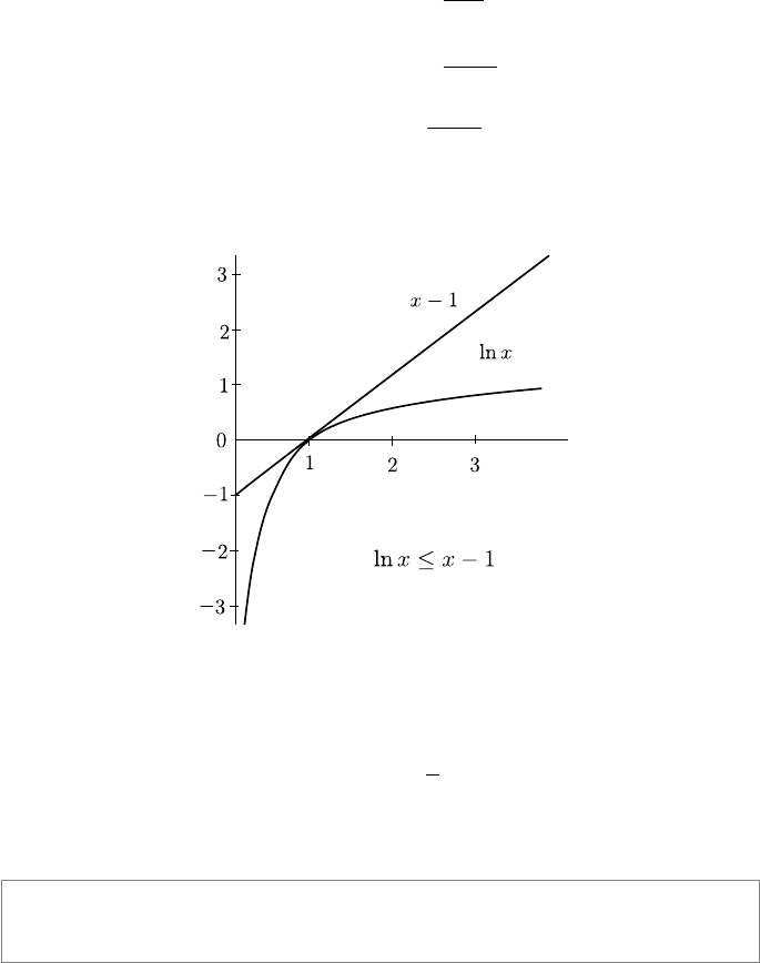
This is because log x ≤ x − 1, with equality only if x = 1 (see Figure 11.2),
an important result often used in information theoretic proofs.
FIGURE 11.2: Graph of y = x − 1 compared with y = ln x.
So we have
H(X) − k log n ≤ k
X
1
n
−
X
p(x)
= 0,
∴ H(X) ≤ k log n. (11.6)
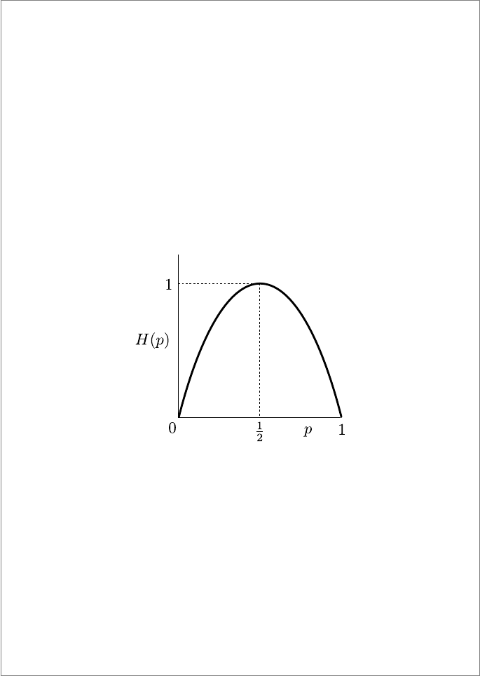
Box 11.1: Binary Entropy
A very useful concept is the entropy function of a probability distribution
218 Introduction to Quantum Physics and Information Processing
of a binary random variable, such as the result of the toss of a coin, not
necessarily unbiased. Here, one value occurs with probability p and the other
with 1 − p. We then have
H
bin
(p) = −p log p − (1 − p) log(1 − p). (11.7)
In this simple case all the listed properties of the mathematical entropy func-
tion are obvious.
1. Positive: H
bin
(p) > 0 always;
2. Symmetric: H
bin
(p) = H
bin
(1 − p);
3. H
bin
(p) has a maximum of 1 when p = 1/2 as in a fair coin;
4. H
bin
(p) has a minimum of 0 when p = 1 as in a two-headed coin.
FIGURE 11.3: The binary entropy function.
This function is a useful tool in deriving properties of entropy, especially when
different probability distributions are mixed together. An important property
of the entropy function is made evident in this simple case: that of concavity.
This property is used very often in concluding various results in classical as
well as quantum information theory. The graph in Figure 11.3 shows that the
function is literally concave. A mathematical statement of this property is
that the function lies above any line cutting the graph. Algebraically, for two
points x
1
, x
2
< 1, we have
H
bin
px
1
+ (1 − p)x
2
≥ pH
bin
(x
1
) + (1 − p)H
bin
(x
2
). (11.8)
Characterization of Quantum Information 219
11.1.3 Relations between entropies of two sets of events
From the way it is defined, Shannon entropy is closely related to probability
theory. In this book, we do not expect a thorough background in probability
theory, so I will simply draw your attention to some important results, so
that you may be piqued enough to look them up on your own. Consider two
ensembles X = {x, p(x)} and Y = {y, p(y)}. We will define various measures
to compare the probability distributions {p(x)} and {p(y)}.
1. Relative entropy of X and Y measures the difference between the two
probability distributions {p(x)} and {p(y)}:
H(X k Y ) = −
X
x,y
p(x) log p(y) − H(X)
=
X
x,y
p(x) log
p(y)
p(x)
. (11.9)
Here again we use the convention that
−0 log 0 ≡ 0, −p(x) log 0 ≡ ∞, p(x) > 0. (11.10)
An important property of the relative entropy is that it is positive. The
relative entropy is also called the Kullback–Leibler distance. However,
it is not symmetric, and so is not a true distance measure, but it gives
us, for example, the error in assuming that a certain random variable
has probability distribution {p(y)} when the true distribution is {p(x)}.
Thus this definition is more useful when we have a set of events X with
two different probability distributions {p(x)} and {q(x)},
H(p k q) =
X
x
p(x) log
p(x)
q(x)
. (11.11)
2. Joint entropy of X and Y measures the combined information pre-
sented by both distributions. Classically, the joint probability of X and
Y , denoted by {p(x, y)}, is defined over a set X ⊗Y . The joint entropy
is then
H(X, Y ) = −
X
x,y
p(x, y) log p(x, y). (11.12)
If X and Y are independent events, then
H(X, Y ) = H(X) + H(Y ). (11.13)
3. Conditional entropy measures the information gained by the occur-
rence of X if Y has already occurred and we know the outcome. The
220 Introduction to Quantum Physics and Information Processing
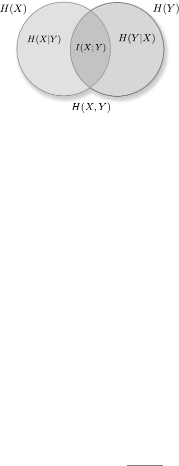
FIGURE 11.4: Relationship between entropic quantities.
classical conditional probability of an event x given y is defined as
p(x|y) = p(x, y)/p(y), and we have
H(X|Y ) = −
X
x,y
p(x|y) log p(x|y) (11.14)
= H(X, Y ) − H(Y ). (11.15)
The second equation is an important relation: a chain rule for entropies:
H(X, Y ) = H(X) + H(Y |X). (11.16)
4. Mutual information measures the correlation between the distribu-
tions of X and Y . This is the difference between the information gained
by the occurrence of X, and the information gained by occurrence of X
if Y has already occurred. The mutual information is symmetric, so we
have
I(X; Y ) = H(X) − H(X|Y ) = H(Y ) − H(Y |X) (11.17)
= H(X) + H(Y ) − H(X, Y ). (11.18)
The mutual information is a measure of how much the uncertainty about
X is reduced by a knowledge of Y . You can also see that it is the relative
entropy of the joint distribution p(x, y) and the product distribution
p(x)p(y):
I(X; Y ) =
X
x,y
p(x, y) log
p(x, y)
p(x)p(y)
. (11.19)
One way to picture the interrelationships between these entropic quantities
is the Venn diagram of Figure 11.4. Given these definitions, the Shannon
entropies satisfy the following properties that are easily proved
Leave a Reply