Basic Energy Balance Problems

A chemical engineer has to perform a wide variety of energy balance computations for a large number of transformations and processes. These computations require application of the principles discussed in section 7.1. The myriad energy balance computations performed by chemical engineers can very broadly be classified into two types: those involving determination of heat effects in particular transformations of interest and those involving determinations of system temperatures as a result of the particular transformation undergone by the system. The following examples provide a brief glimpse into the nature of energy balance computations for different chemical processes.

Example 7.2.1 Adiabatic Flame Temperature of Exhaust Gases

Consider again the material balance discussed in example 6.3.1, the combustion of natural gas. Burning the natural gas releases heat—a manifestation of the principle of the conservation of energy, where the chemical energy stored in methane is converted into chemical energy of products and thermal energy. If this heat is not removed from the system, then it would cause the temperature of the product stream to rise. Adiabatic flame temperature in a combustion process is simply the theoretical temperature reached by the product gases in a combustion process, when the process is conducted adiabatically—without any energy exchange with the surroundings. Calculate the adiabatic flame temperature for complete combustion of natural gas when stoichiometric quantity of air is fed to the burner. All the inlet streams are at 25°C.

Solution

The first step in performing energy balance computations is obtaining the material balance for the process. These material balance calculations were conducted in Chapter 6 and are reproduced in Figure 7.4.

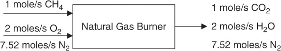
Figure 7.4 Material balance on a natural gas burner.

Note that Figure 7.4 shows the material balance for a continuous process where 1 mol/s of the natural gas is fed to the burner continuously. Since the process is adiabatic, at steady state the enthalpy flowing into the burner must equal the enthalpy leaving the burner:

The enthalpy flowing in is equal to the sum of enthalpies carried into the burner by the three components:

Here,  represents the molar flow rate of component i, and h_i its specific enthalpy (enthalpy per mole).

Similarly, the enthalpy flowing out of the burner is the sum of enthalpies of the components exiting the burner:

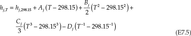
Enthalpies in equations E7.2 and E7.3 are evaluated at the corresponding stream temperatures; that is, at 25°C (298.15 K) for the inlet streams and an unknown temperature T (K) for the product stream. As mentioned earlier, enthalpies at 298.15 K are the enthalpies of formation at the standard state and are available from various sources. The enthalpies h_j can be expressed in terms of this temperature T, making use of equation E7.4:

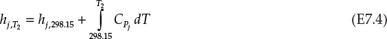
Table E7.1 shows the standard enthalpies of formation (), and Table E7.2 shows the functional dependence of the heat capacity for each component [3, 7].

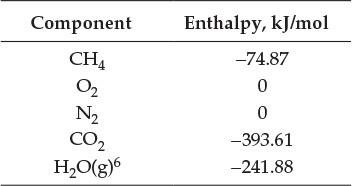
Table E7.1 Standard Enthalpies of Formation

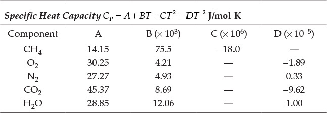
Table E7.2 Functional Dependence of Heat Capacity

Using this data, the rate of enthalpy fed to the system () is found to be equal to -74.87 kJ/s. The rate at which enthalpy is leaving the system is calculated as follows:⁶

6. Gas phase.

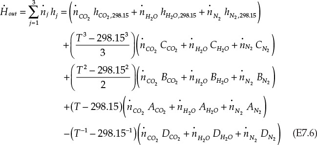
First, the specific enthalpy of each species at temperature T is calculated from the C_P data:

Substituting equation E7.5 in equation E7.3 and rearranging terms gives us the following:

Equation E7.6 appears complicated, but that is primarily because all the individual terms are written in expanded form rather than because of any intrinsic complexity.

The molar flow rates of components in the outlet stream are as shown in Figure 7.4. Equating  to -74.87 kJ/s, and substituting the values of various parameters yields the following equation in unknown outlet temperature T:

Equation E7.7 is a polynomial equation that can be solved using a number of different techniques. The solution using the Goal Seek tool in Microsoft Excel (described in Chapter 5, “Computations in Fluid Flow”) is shown in Figure 7.5.

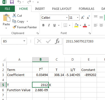
Figure 7.5 Excel Goal Seek solution for adiabatic flame temperature problem.

As seen from the figure, the coefficients of the terms T², T, and 1/T are entered in cells B3, C3, and D3, with the constant value in the cell E3. A temperature guess is provided in cell B5, and the function described by equation E7.7 is evaluated in cell B6. The Goal Seek function manipulates the value in B5 until the function value in B6 is approximately zero. The adiabatic flame temperature is 2312 K (~2039°C).

The graphical solution for the problem using Mathcad is shown in Figure 7.6.

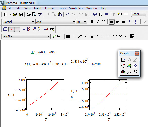
Figure 7.6 Mathcad graphical solution of the adiabatic flame temperature problem.

The steps for obtaining the solution are as follows:

1. First, define a range for variable T by typing T:298.15;2500.

2. Define the function f(T) by typing

f(T):0.03494*T^2 +308.14*T-5.1384*10^5/T-899202

3. Create the graph of f(T) as a function of T by choosing Insert from the command menu, and then Graph and X-Y Plot from the dropdown menus. (Alternatively, a graph can also be created by clicking on the appropriate buttons.) This creates a blank graph with empty placeholders for the x and y variables. Enter T and f(T) by clicking on these placeholders, generating the graph shown at the bottom on the left. As can be seen from the graph, the function value goes from ~-8 × 10⁵ to ~1.6 × 10⁵, indicating that function value is zero in the vicinity of T = 2000. To get an accurate estimate, replot the function, as shown on the right, with the x-axis values between 2300 and 2325. In addition, add a straight horizontal line at y = 0 by clicking at the end of y-axis label f(T) and typing a space followed by 0.

4. The graph on the right clearly shows that the function is zero (from the intersection of the function curve with the horizontal dashed line) at a T value between by 2310 and 2315, enabling a guess for the solution at 2312. Improve the accuracy of the solution by progressively rescaling the x-axis to narrow the limits. However, it should be noted that a solution guess of 2310 is already within 0.1% of the exact solution and is adequate for most practical purposes.

Example 7.2.2 Heat Recovery from Combustion Gases

The combustion gases from the burner in the previous example are cooled to 25°C, in the process heating up water to 150°F (as would happen in a water heater). What is the flow rate of hot water if the cold water entering the heater is at 68°F?

Solution

The schematic of the process is shown in Figure 7.7.

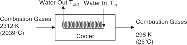
Figure 7.7 Energy balance on a water heater.

As seen from the figure, the water is passed through the inside of the pipe, which is shaped into a coil to provide the necessary area for heat exchange. The energy balance on the process yields the following equation:

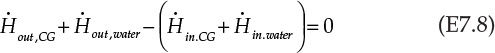
CG stands for combustion gases. Rearranging the terms in Equation E7.8 gives us the following:

Equation E7.9 is the mathematical expression stating that the rate of enthalpy change for combustion gases is exactly equal to the rate of enthalpy change for water; that is, all the energy lost by the combustion gases is transferred to water. An assumption implicit in this statement is that the heater is perfectly insulated and there is no heat loss to the surroundings. The rate of enthalpy flowing in with the combustion gases, , is -74.87 kJ/s, using the information from Example 7.2.1. The other terms in the equation E7.9 are calculated as follows: