
The simplest example of what is called an equation of state is the ideal gas law itself. Equations of state for nonideal gases can be just empirical relations selected to fit a data set, or they can be based on theory, or a combination of the two. Figure 7.4 shows the measurements by Andrews in 1863 of the pressure versus the specific volume for CO2 at various constant temperatures. Note that point C at 31°C is the highest temperature at which liquid and gaseous CO2 can coexist in equilibrium. Above 31°C only critical fluid exists, so that what is called the critical temperature for CO2 is 31°C (304 K). The corresponding gas (fluid) pressure is 72.9 atm (7385 kPa). Also note that at higher temperatures, such as 50°C, the data can be represented by the ideal gas law because pV is constant, a hyperbola. You can find experimental values of the critical temperature (Tc) and the critical pressure (pc) for various compounds on the CD that accompanies this book. If you cannot find a desired critical value in this text or in a handbook, you can consult Reid et al. (refer to the references at the end of this chapter), who describe and evaluate methods of estimating critical constants for various compounds.
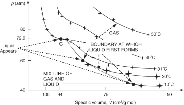
Figure 7.4. Experimental measurements of carbon dioxide by Andrews (+). The solid lines represent smoothed data. C is the highest temperature at which any liquid exists. At the big solid dots liquid and vapor start to coexist. Note the nonlinear scale on the horizontal axis.
How can you predict the p, ![]() , and T properties of a gas between the region in which the ideal gas law is valid and the region in which the gas condenses into liquid? One way is to use one or more equations of state. Where substantial changes in curvature occur, perhaps several different equations must be used to cover a region accurately. Table 7.2 lists some of the well-known single equations of state.
, and T properties of a gas between the region in which the ideal gas law is valid and the region in which the gas condenses into liquid? One way is to use one or more equations of state. Where substantial changes in curvature occur, perhaps several different equations must be used to cover a region accurately. Table 7.2 lists some of the well-known single equations of state.
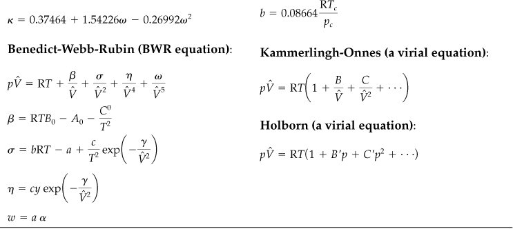
Table 7.2. Examples of Equations of State (for 1 g mol)*
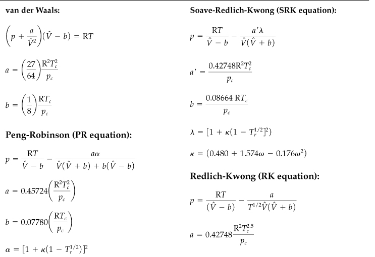
* ![]() is the specific volume, Tc and pc are explained in the text, and ω is the acentric factor, also explained in the text.
is the specific volume, Tc and pc are explained in the text, and ω is the acentric factor, also explained in the text.
The units used in calculating the coefficients in the equations are determined by the units selected for R.
Some of the classical equations of state are formulated as a power series (called the virial form) with p being a function of 1/![]() or
or ![]() being a function of p with three to six terms. You should note that the coefficients in the van der Waals, Peng-Robinson (PR), Soave-Redlich-Kwong (SRK), and Redlich-Kwong (RK) equations can be calculated from certain physical properties (discussed below), whereas in the virial equations the coefficients are strictly determined from experimental measurement. Because of its accuracy, the databases in many commercial process simulators make extensive use of the SRK equation of state. These equations in general will not predict p–
being a function of p with three to six terms. You should note that the coefficients in the van der Waals, Peng-Robinson (PR), Soave-Redlich-Kwong (SRK), and Redlich-Kwong (RK) equations can be calculated from certain physical properties (discussed below), whereas in the virial equations the coefficients are strictly determined from experimental measurement. Because of its accuracy, the databases in many commercial process simulators make extensive use of the SRK equation of state. These equations in general will not predict p–![]() –T values across a phase change from gas to liquid very well. Keep in mind that under conditions such that the gas starts to liquefy, the gas laws apply only to the vapor phase portion of the system for this book.
–T values across a phase change from gas to liquid very well. Keep in mind that under conditions such that the gas starts to liquefy, the gas laws apply only to the vapor phase portion of the system for this book.
How accurate are equations of state? Cubic equations of state such as Redlich-Kwong, Soave-Redlich-Kwong, and Peng-Robinson listed in Table 7.2 can exhibit an accuracy of 1%–2% over a large range of conditions for many compounds. Equations of state in databases may have as many as 30 or 40 coefficients to achieve high accuracy (see, for example, the AIChE DIPPR reports that can be located on the AIChE Web site). Keep in mind that you must know the region of validity of any equation of state and not extrapolate outside that region, particularly not into the liquid region, by ignoring the possibility of condensation for gases such as CO2, NH3, and low-molecular-weight organic compounds such as acetone, ethyl alcohol, and so on. If you plan to use a specific equation of state such as one of those listed in Table 7.2, you have numerous choices, no one of which will consistently give the best results.
Although this may seem a paradox, all exact science is dominated by the idea of approximation.
Bertrand Russell
Other than the use of equations of state to make predictions of values of p, ![]() , and T, what good are they?
, and T, what good are they?
1. They permit a concise summary of a large mass of experimental data and also permit accurate interpolation between experimental data points.
2. They provide a continuous function to facilitate calculation of physical properties based on differentiation and integration of p–![]() –T relationships.
–T relationships.
3. They provide a point of departure for the treatment of the properties of mixtures.
In addition, some of the advantages and disadvantages of using equations of state versus other methods to make predictions are the following:
Advantages:
1. Values of p–![]() –T can be predicted with reasonable error in regions where no data exist.
–T can be predicted with reasonable error in regions where no data exist.
2. Only a few values of coefficients are needed in the equation to be able to predict gas properties, versus collecting large amounts of data by experiment for tables and graphs.
3. The equations can be manipulated on a computer whereas graphics methods of prediction cannot.
Disadvantages:
1. The form of an equation is hard to change to fit new or better data.
2. Inconsistencies may exist between equations for p–![]() –T and equations for other physical properties.
–T and equations for other physical properties.
3. Usually the equation is quite complicated and may not be easy to solve for p, ![]() , or T because of its nonlinearity.
, or T because of its nonlinearity.
I consider that I understand an equation when I can predict the properties of its solutions, without actually solving it.
Paul Dirac
Disadvantage 3 prevented the widespread use of equations of state until computers and computer programs for solving nonlinear algebraic equations came into the picture. You can see that it is easy to solve the SRK equation in Table 7.2 for p given values for T and ![]() , or for T given values of p and
, or for T given values of p and ![]() , but quite difficult and tedious to solve for
, but quite difficult and tedious to solve for ![]() given values for T and p without the aid of computers. Similar remarks apply to virial equations.
given values for T and p without the aid of computers. Similar remarks apply to virial equations.
For example, look at the Redlich-Kwong (RK) equation. Given p and T, is the RK equation cubic in ![]() ? Yes. Given p, T, and
? Yes. Given p, T, and ![]() , is the RK equation cubic in n? Yes. Given p and
, is the RK equation cubic in n? Yes. Given p and ![]() , is it cubic in T? No. We will not focus in this book on how to solve cubic and more complex equations for
, is it cubic in T? No. We will not focus in this book on how to solve cubic and more complex equations for ![]() but instead use an equation solver such as Polymath on the CD in the back of the book.
but instead use an equation solver such as Polymath on the CD in the back of the book.
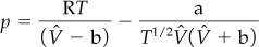
Example 7.6. Use of the RK Equation to Calculate p or ![]()
Determine the pressure (in atmospheres) of 1 g mol of C2H4 at 300 K with V = 0.674 L using the RK equation. From the CD that accompanies the book, for C2H4: Tc = 282.8 K and pc = 50.44 atm.
Solution
The RK equation is (from Table 7.2)
What should you do first? Take a basis of the given values of V, n, and T. Then calculate a, b, and ![]()
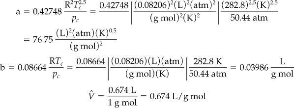
Next, insert the known values of the variables and coefficients:
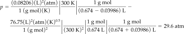
If you know p and V instead of p and T, you can solve explicitly for T by rearranging the equation or by using an equation solver. Figure E7.6 compares the prediction of p by the ideal gas law and the RK equation.
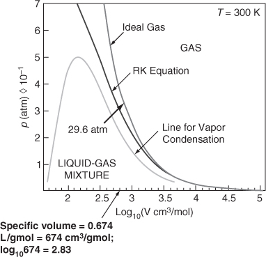
Figure E7.6
Next, let’s determine the specific volume of C2H4 at 300 K and 30 atm using the RK equation. Because with the RK equation you cannot explicitly solve for ![]() , what should you do now? You can solve the RK equation in the usual format after introducing the known values and then use Polymath to determine
, what should you do now? You can solve the RK equation in the usual format after introducing the known values and then use Polymath to determine ![]() = 0.6748 L/g mol.
= 0.6748 L/g mol.
7.2.2. The Critical State and Compressibility
We mentioned the critical pressure pc and critical temperature Tc in connection with Figure 7.4. The critical state (point) for the gas-liquid transition is the set of physical conditions at which the density and other properties of the liquid and vapor become identical. In Figure 7.5 the points on the constant temperature lines at which the gas (vapor) starts to condense have been connected by a dashed line (—). On the opposite side of the figure, the dot-dashed curve (___ . ___) shows the locus of points at the respective temperatures at which completion of the condensation occurs; that is, the vapor becomes all liquid. Between the two bounds a mixture of vapor and liquid exists.
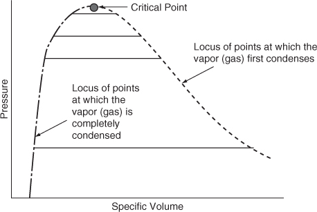
Figure 7.5. The critical point is located where the lengths of the (solid) lines are zero. The solid lines connect the points at which condensation starts at various temperatures to the corresponding points for that temperature at which condensation is complete.
The intersection of the two bounds is denoted as the critical point, and it occurs at the highest temperature and pressure possible (Tr = 1, pr = 1) at which gas and liquid can coexist.
A supercritical fluid is a compound in a state above its critical point. Supercritical fluids are used to replace solvents such as trichloroethylene and methylene chloride, the emissions from which, and the contact with which, have been severely limited. For example, coffee decaffeination, the removal of cholesterol from egg yolk with CO2, the production of vanilla extract, and the destruction of undesirable organic compounds all can take place using supercritical water. Supercritical water has been shown to destroy 99.99999% of all of the major types of toxins in these organic compounds.
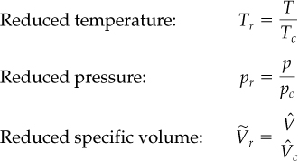
Other terms with which you should become familiar are the reduced variables. These are conditions of temperature, pressure, or specific volume normalized (divided) by their respective critical conditions, as follows:
In theory, the law of corresponding states indicates that any compound should have the same reduced volume at the same reduced temperature and reduced pressure so that a universal gas law might be

Unfortunately Equation (7.7) does not universally make accurate predictions. You can check this conclusion by selecting a compound such as water, applying Equation (7.7) at some low temperature and high pressure to calculate ![]() , and comparing your results with the value obtained for
, and comparing your results with the value obtained for ![]() with the corresponding conditions from the tables for water vapor that are in the folder in the back of this book.
with the corresponding conditions from the tables for water vapor that are in the folder in the back of this book.
The concept of reduced variables nevertheless has been applied to prediction of real gas properties. One common way is to modify the ideal gas law by inserting an adjustable coefficient z, the compressibility factor, a factor that compensates for the nonideality of the gas, and can be looked at as a measure of nonideality. Thus, the ideal gas law is turned into a real gas law called a generalized equation of state:

or

One way to look at z is to consider it to be a factor that makes Equation (7.8) an equality. Note that z = 1 is for an ideal gas. Although we treat only gases in this chapter, Equation (7.8) has been applied to liquids.
If you plan on using Equation (7.8), where can you find the values of z to use in it? Equations exist in the literature for specific compounds and classes of compounds, such as those found in petroleum refining. Theoretical calculations based on molecular structure sometimes prove to be useful. Refer to the references at the end of this chapter. Usually you will find graphs or tables of z to be quite convenient sources for engineering purposes. If the compressibility factor derived from experiment is plotted for a given temperature against the pressure for different gases, figures such as Figure 7.6a result. However, if the compressibility factor is plotted against the reduced pressure as a function of the reduced temperature, then for like gases the compressibility values at the same reduced temperature and reduced pressure fall at about the same point, as illustrated in Figure 7.6b.
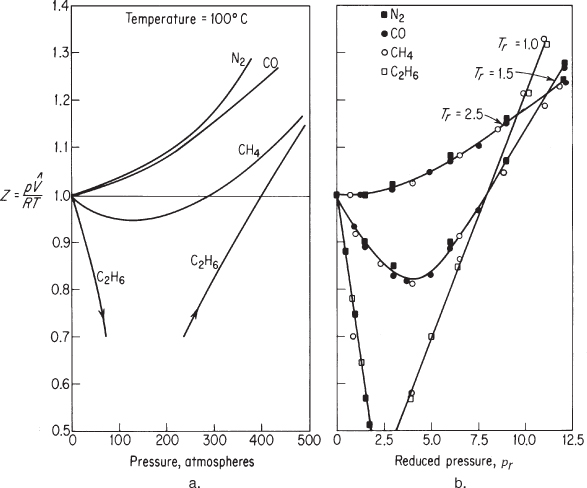
Figure 7.6. (a) Compressibility at 100°C for several gases as a function of pressure; (b) compressibility factor for several gases as a function of reduced temperature and reduced pressure
You can use the charts described in the next section, Section 7.3, to get approximate values of z as a function of the reduced temperature and pressure. Or, you can use one of the numerous methods that have appeared in the literature and in process simulation codes to calculate z via an equation in order to obtain more accurate values of z than can be obtained from charts. Equation (7.9) employs the Pitzer acentric factor, ω:

Tables in Appendix C list values of z0 and z1 as a function of Tr and pr; ω is unique for each compound, and you can find values for it on the CD that accompanies this book. Table 7.3 is an abbreviated table of the acentric factors from Pitzer.
Table 7.3. Selected Values of the Pitzer* Acentric Factor
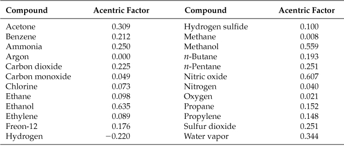
*K. S. Pitzer, J. Am. Chem. Soc., 77, 3427 (1955).
The acentric factor ω indicates the degree of acentricity or nonsphericity of a molecule. For helium and argon, ω is equal to zero. For higher-molecular-weight hydrocarbons and for molecules with increased polarity, the value of ω increases.
As an example of calculating z via the Pitzer correlation, calculate the compressibility factor z for ethylene (C2H4) at 300 K and 3000 kPa. First get Tc (283.1 K) and pc (50.5 atm) from the CD, and then calculate Tr and pr:
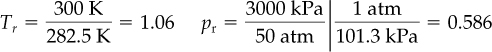
Next, look up (using interpolation) z0 (0.812) and z1(–0.01) as well as ω (0.089) from Appendix C or Table 7.3.
z = 0.812 + (–0.01)(0.089) = 0.812
The calculation of z is easy if you know the values of p and T for the gas and just want to calculate z for those two conditions. But if you know p and ![]() or T and
or T and ![]() , you have to employ a trial-and-error solution to get z. What you do is assume a sequence of values of p, calculate the related sequence of values of pr, and next calculate the associated sequence of values of z. Then you calculate values of
, you have to employ a trial-and-error solution to get z. What you do is assume a sequence of values of p, calculate the related sequence of values of pr, and next calculate the associated sequence of values of z. Then you calculate values of ![]() from p
from p![]() = zRT. When you find the value of the specific volume that matches the value specified in the problem, you have an appropriate z (and
= zRT. When you find the value of the specific volume that matches the value specified in the problem, you have an appropriate z (and ![]() ).
).
A different way of predicting p, ![]() , and T properties is the group contribution method which has been successful in estimating properties of pure components. This method is based on combining the contribution of each functional group of a compound. The key assumption is that a group such as –CH3 or –OH behaves identically irrespective of the molecule in which it appears. This assumption is not quite true, so any group contribution method yields approximate values for gas properties. Probably the most widely used group contribution method is UNIFAC,1 which forms a part of many computer databases. UNIQUAC is a variant of UNIFAC and is widely used in the chemical industry in the modeling of nonideal systems (systems with strong interaction between the molecules).
, and T properties is the group contribution method which has been successful in estimating properties of pure components. This method is based on combining the contribution of each functional group of a compound. The key assumption is that a group such as –CH3 or –OH behaves identically irrespective of the molecule in which it appears. This assumption is not quite true, so any group contribution method yields approximate values for gas properties. Probably the most widely used group contribution method is UNIFAC,1 which forms a part of many computer databases. UNIQUAC is a variant of UNIFAC and is widely used in the chemical industry in the modeling of nonideal systems (systems with strong interaction between the molecules).
Self-Assessment Test
Questions
1. Explain why the van der Waals and Peng-Robinson equations (of state) are easy to solve for p and hard to solve for V.
2. Under what conditions will an equation of state be the most accurate?
3. What are the units of a and b in the SI system for the Redlich-Kwong equation?
Problems
1. Convert the virial (power series) equations of Kammerlingh-Onnes and Holborn (in Table 7.2) to a form that yields an expression for z.
2. Calculate the temperature of 2 g mol of a gas using van der Waals’ equation with a = 1.35 × 10⁻⁶ m6 (atm)(g mol–2), b = 0.0322 × 10⁻³ (m3)(g mol–1) if the pressure is 100 kPa and the volume is 0.0515 m3.
3. Calculate the pressure of 10 kg mol of ethane in a 4.86 m3 vessel at 300 K using two equations of state: (a) ideal gas and (b) Soave-Redlich-Kwong. Compare your answer with the experimentally observed value of 34.0 atm.
Thought Problems
1. Data pertaining to the atmosphere on Venus (which has a gravitational field only 0.81 that of the Earth) shows that the temperature of the atmosphere at the surface is 474 ± 20°C and the pressure is 90 ± 15 atm. What do you think is the reason(s) for the difference between these figures and those at the Earth’s surface?
2. A method of making protein nanoparticles (0.5 to 5.0 μ in size) has been patented by the Aphio Corp. Anti-cancer drugs that small can be used in novel drug delivery systems. In the process described in the patent, protein is mixed with a gas such as carbon dioxide or nitrogen at ambient temperature and 20,000 kPa pressure. When the pressure is released, the proteins break up into fine particles.
What are some of the advantages of such a process versus making powders by standard methods?
Discussion Question
Fossil fuels provide most of our power, and the carbon dioxide produced is usually discharged to the atmosphere. The Norwegian company Statoil separates carbon dioxide from its North Sea gas production and, since 1996, has been pumping it at the rate of 1 million tons per year into a layer of sandstone 1 km below the seabed. The sandstone traps the gas in a gigantic bubble that in 2001 contained 4 million tons of carbon dioxide.
Will the bubble of carbon dioxide remain in place? What problems exist with regard to the continuous addition of carbon dioxide in future years? Is the carbon dioxide actually a gas?
Leave a Reply