
In Section 7.3, we discussed vapor-liquid equilibria of a pure component. In Section 7.4, we covered equilibria of a pure component in the presence of a noncondensable gas. In this section, we consider certain aspects of a more general set of circumstances, namely, cases in which both the liquid and vapor have two components; that is, the vapor and liquid phases each contain both components. Distilling moonshine from a fermented grain mixture is an example of binary vapor-liquid equilibrium in which water and ethanol are the primary components in the system and are present in both the vapor and the liquid.
The primary result of vapor-liquid equilibrium is that the more volatile component (i.e., the component with the larger vapor pressure at a given temperature) tends to accumulate in the vapor phase while the less volatile component tends to accumulate in the liquid phase. Distillation columns, which are used to separate a mixture into its components, are based on this principle. A distillation column is composed of a number of trays that provide contacting between liquid and vapor streams inside the column. At each tray, the concentration of the more volatile component is increased in the vapor stream leaving the tray, and the concentration of the less volatile component is increased in the liquid leaving the tray. In this manner, applying a number of trays in series, the more volatile component is concentrated in the overhead stream from the column while the less volatile component is concentrated in the bottom product. In order to design and analyze distillation, you must be able to quantitatively describe vapor-liquid equilibrium for these systems.
7.5.1 Ideal Solution Relations
An ideal solution is a mixture whose properties such as vapor pressure, specific volume, and so on can be calculated from the knowledge of only the corresponding properties of the pure components and the composition of the solution. For a solution to behave as an ideal solution:
- All of the molecules of all types should have the same size.
- All of the molecules should have the same intermolecular interactions.
Most solutions are not ideal, but some real solutions are nearly ideal.
Raoult’s law
The best-known relation for ideal solutions ispi=xipi*(T)
(7.8)
wherepi=partial presure of component i in the vapor phasexi=mole fraction of component i in the liquid phasepi*(T)=vapor pressure of component i at T
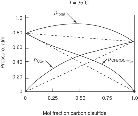
Figure 7.15 shows how the vapor pressure of the two components in an ideal binary solution sum to the total pressure at 80°C. Compare Figure 7.15 with Figure 7.16, which displays the pressures for a nonideal solution.
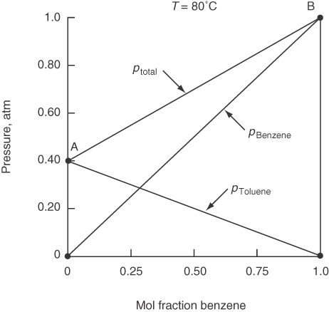
Raoult’s law is used primarily for a component whose mole fraction spans the full range from 0 to 1 for solutions of components quite similar in chemical nature, such as straight-chain hydrocarbons.
Henry’s law
Henry’s law is used primarily for a component whose mole fraction approaches zero, such as a dilute gas dissolved in a liquid:pi=Hixi
(7.9)
where pi is the partial pressure in the gas phase of the dilute component at equilibrium at some temperature, and Hi is the Henry’s law constant. Note that in the limit where xi → 0, pi → 0. Values of Hi can be found in several handbooks and on the Internet.
Henry’s law is quite simple to apply when you want to calculate the partial pressure of a gas that is in equilibrium with the gas dissolved the liquid phase. Take, for example, CO2 dissolved in water at 40°C for which the value of H is 69,600 atm/mol fraction. (The large value of H shows that CO2(g) is only sparing soluble in water.) If xCO2 = 4.2 × 10⁻⁶, the partial pressure of the CO2 in the gas phase is
pCO2 = 69,600(4.2 × 10⁻⁶) 0.29 atm
That is, the gas phase contains almost 30% CO2 for 1 atm pressure, but the liquid phase would contain only 0.00042% CO2.
7.5.2 Vapor-Liquid Equilibria Phase Diagrams
The phase diagrams discussed in Section 7.2 for a pure component can be extended to cover binary mixtures. Experimental data usually are presented as pressure as a function of composition at a constant temperature, or temperature as a function of composition at a constant pressure. For a pure component, vapor-liquid equilibrium occurs with only one degree of freedom:
F = 2 − P + C = 2 − 2 + 1 = 1
At 1 atm pressure, vapor-liquid equilibrium will occur at only one temperature: the normal boiling point. However, if you have a binary solution, you have two degrees of freedom:
F = 2 − 2 + 2 = 2
For a system at a fixed pressure, both the phase compositions and the temperature can be varied over a finite range. Figures 7.17 and 7.18 show the vapor-liquid envelope for a binary mixture of benzene and toluene, which is essentially ideal.
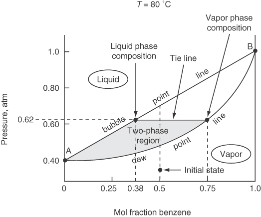
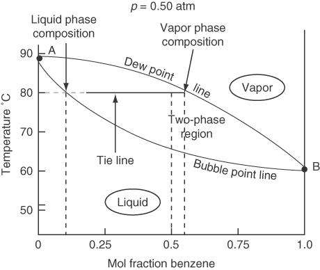
You can interpret the information on the phase diagrams as follows: Suppose you start in Figure 7.17 at a 50-50 mixture of benzene-toluene at 80°C and 0.30 atm in the vapor phase. Then you increase the pressure on the system until you reach the dew point at about 0.47 atm, at which point the vapor starts to condense. At 0.62 atm the mole fraction in the vapor phase will be about 0.75, and the mole fraction in the liquid phase will be about 0.38 as indicated by the tie line. As you increase the pressure from 0.70 atm, all of the vapor will have condensed to liquid. What will the composition of the liquid be? 0.50 benzene, of course! Can you carry out an analogous conversion of vapor to liquid on Figure 7.18, the temperature-composition diagram?
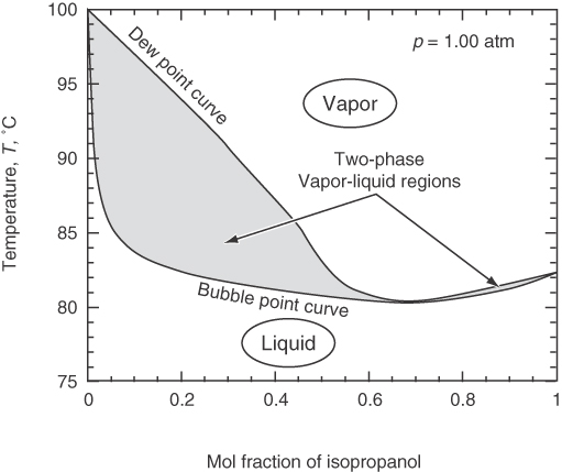
Phase diagrams for nonideal solutions abound. Figure 7.19 shows the temperature-composition diagram for isopropanol in water at 1 atm. Note the minimum boiling point at a mole fraction of isopropanol of about 0.68, a point called an azeotrope (a point at which on a yi-versus-xi plot the function of (yi/xi) crosses the function yi = xi, a straight line). An azeotrope makes separation by simple distillation difficult because it creates a pinch point because when the dew point and the bubble point coincide so that separation between the more volatile and the less volatile components does not occur.
7.5.3 K-value (Vapor-Liquid Equilibrium Ratio)
For nonideal as well as ideal mixtures that comprise two (or more) phases, it proves to be convenient to express the ratio of the mole fraction in one phase to the mole fraction of the same component in another phase in terms of a distribution coefficient or equilibrium ratio K, usually called a K-value. For example:Vapor-liquid ratio of component i=yixi=Ki
(7.10)
and so on. If the ideal gas law pi = yi ptotal applies to the gas phase and the ideal Raoult’s law pi=xipi*(T) applies to the liquid phase, then for an ideal systemKi=yixi=pi*(T)ptotal
(7.10a)
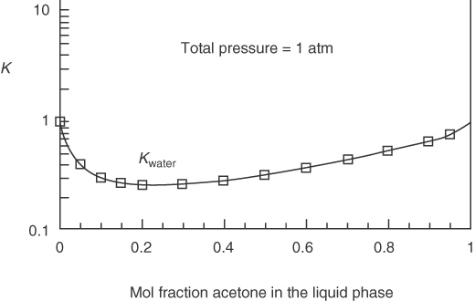
Equation (7.10a) gives reasonable estimates of Ki values at low pressures for components well below their critical temperatures but yields values too large for components above their critical temperatures, at high pressures, and/or for polar compounds. For nonideal mixtures, Equation (7.10) can be employed if Ki is made a function of temperature, pressure, and composition so that relations for Ki can be fit by equations to experimental data and used directly, or in the form of charts, for design calculations, as explained in some of the references at the end of this chapter. Figure 7.20 shows how K varies for the nonideal mixture of acetone and water at 1 atm. K can be greater or less than 1 but never negative.
For ideal solutions, you can calculate values of K using Equation (7.10a). For nonideal solutions you can get approximate K-values from
- Empirical equations such as44S. I. Sandler, in Foundations of Computer Aided Design, Vol. 2, edited by R. H. S. Mah and W. D. Seider, American Institute of Chemical Engineers, New York (1981), p. 83.If Tc,i/T >1.2: Ki=(pc,i)exp[7.224−7.534/Tr.i−2.598 ln Tr,i]ptotal
- Databases refer to the supplementary references (at the end of the chapter).
- Charts such as Figure 7.21
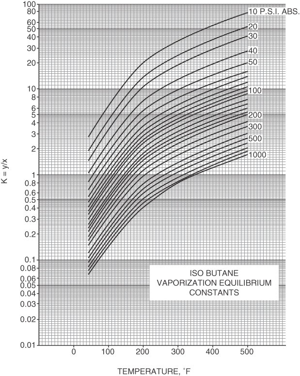 Figure 7.21 K-values for isobutane as a function of temperature and pressure. From Natural Gasoline Association of America Technical Manual, 4th ed. (1941) (based on data provided by George Granger Brown).
 - Thermodynamic relations refer to the references (at the end of the chapter).
7.5.4 Bubble Point and Dew Point Calculations
Here are some typical problems you should be able to solve that involve the use of the equilibrium coefficient Ki and material balances:
1. Calculate the bubble point temperature of a liquid mixture given the total pressure and liquid composition.
To calculate the bubble point temperature (given the total pressure and liquid composition), you can write Equation (7.10) as yi = Kixi. Also, you know that Σyi = 1 in the vapor phase. Thus, for a binary,1=K1x1+K2x2
(7.11)
in which the Ki are functions of solely the temperature. Because each of the Ki increases with temperature, Equation (7.11) has only one positive root. A trial-and-error procedure is required to determine the bubble point temperature, which can be performed on the computer or by hand. If you choose to solve for the bubble point by hand, you have to assume varying temperatures so that you can look up or calculate Ki, and then calculate each term in Equation (7.11). After the sum (K1x1 + K2x2) brackets 1, you can interpolate to get a T that satisfies Equation (7.11).
For an ideal solution, Equation (7.11) becomesptotal=p1*x1+p2*x2
(7.12)
and you might use Antoine’s equation for p*i. Once the bubble point temperature is determined, the vapor composition can be calculated fromyi=pi*xiptotal
A degree-of-freedom analysis for the bubble point temperature for a binary mixture shows that the degrees of freedom are zero:
Total variables=2×2+2=6variables:x1, x2; y1, y2; ptotal; T
Prespecified values of = 2 + 1 = 3 variables: x1, x2; pTotalIndependent equations=2+1=3 equations: y1=K1x1, y2=K2x2; y1+y2=1
Therefore, there are three unknowns and three equations with which to determine their values.
2. Calculate the dew point temperature of a vapor mixture given the total pressure and vapor composition.
To calculate the dew point temperature (given the total pressure and vapor composition), you can write Equation (7.10) as xi = yi/Ki, and you know Σxi = 1 in the liquid phase. Consequently, you want to solve the equation1=y1K1+y2K2
(7.13)
in which the Ks are functions of temperature as explained for the bubble point temperature calculation. For an ideal solution,1=ptotal[y1p1*+y2p2*]
(7.13a)
The degree-of-freedom analysis is similar to that for the bubble point temperature calculation.
In selecting a particular form of the equation to be used for your equilibrium calculations, you must select a method of solving the equation that has desirable convergence characteristics. Convergency to the solution should
- Lead to the desired root if the equation has multiple roots
- Be stable, that is, approach the desired root asymptotically rather than by oscillating
- Be rapid, and not become slower as the solution is approached
You can use MATLAB’s fzero function or Python’s scipy.optimize.newton, which were introduced in Chapter 6, Section 6.2.2, to solve bubble point and dew point equations because in both cases the equation to be solved is a single nonlinear equation in which the temperature is unknown. These equations can be more efficiently and reliably solved by first transforming them into a more linear form.5
5 J. B. Riggs, Computational Methods for Chemical Engineers (Austin, TX: Ferret Publishing, 2020), 95–97.
Table 7.1 summarizes the usual phase equilibrium calculations.
Table 7.1 Summary of the Information Associated with Typical Phase Equilibrium Calculations
| Type | Known* Information | Variables to Be Calculated | Equation(s) to Use | Convergence Characteristics |
|---|---|---|---|---|
| Bubble point temperature | ptotal, xi | T, yi | 7.10 | Good |
| Dew point temperature | ptotal, yi | T, xi | 7.12 | Good |
| Bubble point pressure | T, xi | ptotal, yi | 7.10 | Fair |
| Dew point pressure | T, yi | ptotal, xi | 7.12 | Fair |
* Ki is assumed to be a known function of T, p, and composition
Leave a Reply