Main Concepts

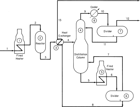
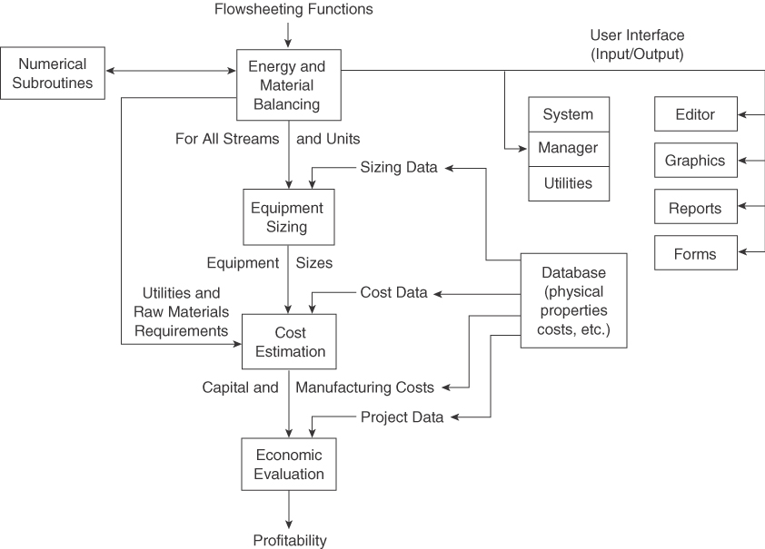
As explained in Chapter 6, a plant flowsheet such as the simple diagram in Figure 14.1 mirrors the stream network and equipment arrangement in a process. Once the process flowsheet is specified, or during its formulation, the solution of the appropriate process material and energy balances is referred to as process simulation or flowsheeting, and the computer code used in the solution is known as a process simulator or flowsheeting code. Codes for both steady-state and dynamic processes exist. The essential problem in flowsheeting is to solve (satisfy) a large set of linear and nonlinear equations and constraints to an acceptable degree of precision. Such a program can also, at the same time, determine the size of equipment and piping, evaluate costs, and optimize performance. Figure 14.2 shows the information flow that occurs in a process simulator.

The software must facilitate the transfer of information between equipment and streams, have access to a reliable database, and be flexible enough to accommodate equipment specifications provided by the user to supplement the library of programs that come with the code. Fundamental to all flowsheeting codes is the calculation of mass and energy balances for the entire process. Valid inputs to the material and energy balance phase of the calculations for the flowsheet must be defined in sufficient detail to determine all of the intermediate and product streams and the unit performance variables for all units.

Frequently, process plants contain recycle streams and control loops, and the solution for the stream properties requires iterative calculations. Thus, efficient numerical methods must be used. In addition, appropriate physical properties and thermodynamic data have to be retrieved from a database. Finally, a master program must exist that links all of the building blocks, physical property data, thermodynamic calculations, subroutines, and numerical subroutines, and that also supervises the information flow. You will find that optimization and economic analysis are often the ultimate goals in the use of flowsheeting codes.

Other specific applications include

1. Steady- and unsteady-state simulation to help improve and verify the design of a process and examine complicated or dangerous designs
2. Training of operators
3. Data acquisition and reconciliation
4. Process control, monitoring, diagnostics, and troubleshooting
5. Optimization of process performance
6. Management of information
7. Safety analysis

Typical unit process models found in process simulators for both steady-state and unsteady-state operations include

1. Reactors of various kinds
2. Phase separation equipment
3. Ion exchange and absorption
4. Drying
5. Evaporation
6. Pumps, compressors, blowers
7. Mixers, splitters
8. Heat exchangers
9. Solid-liquid separators
10. Solid-gas separators
11. Storage tanks

Features that you will find in a general process simulator include

1. Unit and equipment models representing operations and procedures
2. Software to solve material and energy balances
3. An extensive database of physical properties
4. Equipment sizing and costing functions
5. Scheduling of batch operations
6. Environmental impact assessment
7. Compatibility with auxiliary graphics, spreadsheets, and word-processing functions
8. Ability to import and export data

Table 14.1 lists some commercial process simulators.

From the viewpoint of a user of a process simulator code you should realize:

Table 14.1 Vendors of Commercial Process Simulators

Name of Program	Source
ABACUSS II	MIT, Cambridge, MA
Aspen Engineering Suite (AES)	Aspen Technology, Cambridge, MA
CHEMCAD	Chemstations, Houston, TX
DESIGN II	WinSim, Houston, TX
D-SPICE	Fantoft Process Technologies, Houston, TX
HYSIM, HYSYS	Hyprotech, Calgary, Alberta
PRO/II, PROTISS	Simulation Sciences, Fullerton, CA
ProSim	Bryan Research and Engineering, Bryan, TX
SPEEDUP	Aspen Technology Corp., Cambridge, MA
SuperPro Designer	Intelligen, Scotch Plains, NJ

1. Several levels of analysis can be carried out beyond just solving material balances, including solving material plus energy balances, determining equipment sizing, profitability analysis, and much more. Crude, approximate flowsheets are usually studied before fully detailed flowsheets.
2. The results obtained by simulation rest heavily on the type and validity of the choices you make in the selection of the physical property package to be used.
3. You have to realize that the basic function of the process simulator is to solve equations. In spite of the progress made in equation solvers in the last 50 years, the information structure you introduce into the code may yield erroneous or no results. Check essential results by hand. Limits introduced on the range of variables must be valid.
4. A learning curve exists in using a process simulator so that initially a simple problem may take hours to solve, whereas as your familiarity with the simulator increases, it may take only minutes to solve the same problem.
5. GIGO (Garbage In Garbage Out). You have to take care to put appropriate data and connections between units into the data files for the code. Some diagnostics are provided, but they cannot troubleshoot all of your blunders.

Two extremes exist in process simulator software. At one extreme, the entire set of equations (and inequalities) representing the process is written down, including the material and energy balances, the stream connections, and the relations representing the equipment functions. This representation is known as the equation-oriented method of flowsheeting. The equations can be solved in a sequential fashion analogous to the modular representation described below, or simultaneously by Newton’s method (or the equivalent), or by employing sparse matrix techniques to reduce the extent of matrix manipulations; you can find specific details in the references at the end of this chapter.

At the other extreme, the process can be represented by a collection of modules (the modular method of flowsheeting) in which the equations (and other information) representing each subsystem or piece of equipment are collected together and coded so that the module may be used in isolation from the rest of the flowsheet and hence is portable from one flowsheet to another, or can be used repeatedly in a given flowsheet. A module is a model of an individual element in a flowsheet (such as a reactor) that can be coded, analyzed, debugged, and interpreted by itself. In its usual formulation it is an input-output model; that is, given the input values, the module calculates the output values, but the reverse calculation is not feasible. Units represented solely by equations sometimes can yield inputs given the outputs. Some modular-based software codes such as Aspen Plus integrate equations with modules to speed up the calculations.

Another classification of flowsheeting codes focuses on how the equations or modules are solved. One treatment is to solve the equations or modules sequentially, and the other is to solve them simultaneously. Either the program and/or the user must select the decision variables for recycle and provide estimates of certain stream values to make sure that convergence of the calculations occurs, especially in a process with many recycle streams.

A third classification of flowsheeting codes is whether they solve steady-state or dynamic problems. We consider only the former here.

We will review equation-based process simulators first, although historically modular-based codes were developed first, because they are much closer to the techniques described up to this point in this book, and then turn to consideration of modular-based flowsheeting.

14.1.1 Equation-Based Process Simulation

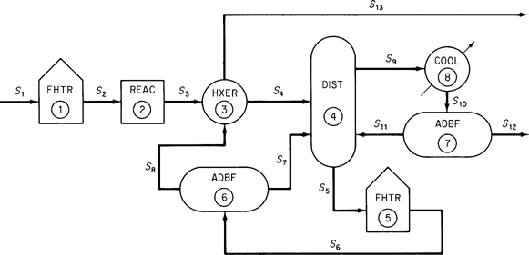
Sets of linear and/or nonlinear equations can be solved simultaneously using an appropriate computer code. Equation-based flowsheeting codes have some advantages in that the physical property data needed to obtain values for the coefficients in the equations are transparently transmitted from a database at the proper time in the sequence of calculations. Figure 14.3 shows the information flow corresponding to the flowsheet in Figure 14.1.

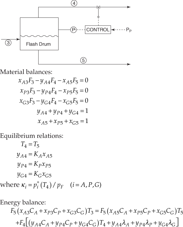
Figure 14.4 is a set of equations that represents the basic operation of a flash drum.

The interconnections between the unit modules may represent information flow as well as material and energy flow. In the mathematical representation of the plant, the interconnection equations are the material and energy balance flows between model subsystems. Equations for models such as mixing, reaction, heat exchange, and so on must also be listed so that they can be entered into the computer code used to solve the equation. Figure 14.5 (and Table 14.2) lists the common types of equations that might be used for a single subsystem.

In general, similar process units repeatedly occur in a plant and can be represented by the same set of equations that differ only in the names of variables, the number of terms in the summations, and the values of any coefficients in the equations.

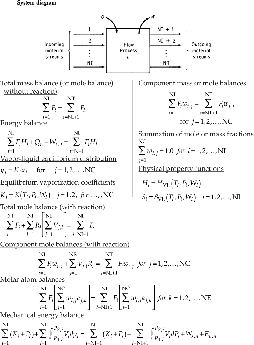
Table 14.2 Notation for Figure 14.5

aj,k	Number of atoms of the kth chemical element in the jth component
Fi	Total flow rate of the ith stream
Hi	Relative enthalpy of the ith stream
Kj	Vaporation coefficient of the jth component
NC	Number of chemical components (compounds)
NE	Number of chemical elements
NI	Number of incoming material streams
NR	Number of chemical reactions
NT	Total number of material streams
pi	Pressure of the ith stream
Qn	Heat transfer for the nth process unit
Rl	Reaction expression for the lth chemical reaction
Ti	Temperature of the ith stream
Vj,l	Stoichiometric coefficient of the jth component in the lth chemical reaction
wi,j	Fractional composition (mass of mole) of the jth component in the ith stream
W¯i	Average composition in the ith stream
Ws,n	Work for the nth process unit
xj	Mole fraction of component j in the liquid
yj	Mole fraction of component j in the vapor

Equation-based codes can be formulated to include inequality constraints along with the equations. Such constraints might be of the form a₁x₁ + a₂x₂ + . . . ≤ b and might arise from such factors as

1. Conditions imposed in linearizing any nonlinear equations
2. Process limits for temperature, pressure, concentration
3. Requirements that variables be in a certain order
4. Requirements that variables be positive or integer

As you can see from Figures 14.4 and 14.5, if all of the equations for the material and energy balances plus the phase and chemical equilibrium relationships plus the thermodynamic and kinetic relations are combined, they form a huge, sparse (few variables in any equation) array. The set of equations can be partitioned into subsets of equations that cannot further be decomposed and have to be solved simultaneously. Two important aspects of solving the sets of nonlinear equations in flowsheeting codes, both equation-based and modular, are (1) the procedure for establishing the precedence order in solving the equations, and (2) the treatment of recycle (feedback) of information, material, and/or energy. Details of how to accommodate these important issues efficiently can be found in the references at the end of this chapter.

Whatever the process simulator used to solve material and energy balance problems, you must provide certain input information to the code in an acceptable format. All flowsheeting codes require that you convert the information in the flowsheet (see Figure 14.1) and the information flowsheet as illustrated in Figure 14.3, or something equivalent. In the information flowsheet, you use the name of the mathematical model (or the subroutine in modular-based flowsheeting) that will be used for the calculations instead of the name of the process unit.

Once the information flowsheet is set up, the determination of the process topology is easy; that is, you can immediately write down the stream interconnections between the modules (or subroutines) that have to be included in the input data set. For Figure 14.3 the matrix of stream connections (the process matrix) is (a negative sign designates an exit stream):

Unit	Associated Streams
1	1	−2
2	2	−3
3	3	8	−4	−13
4	4	7	11	−9	−5
5	5	−6
6	6	−8	−7
7	10	−11	−12
8	9	−10