
The collector performance test is performed under steady-state conditions, with steady radiant energy falling on the collector surface, a steady fluid flow rate, and constant wind speed and ambient temperature. When a constant inlet fluid temperature is supplied to the collector, it is possible to maintain a constant outlet fluid temperature from the collector. In this case, the useful energy gain from the collector is calculated from:
![]() (4.2)
(4.2)
From Chapter 3, we have seen that the useful energy collected from a solar collector is given by:
![]() (4.3)
(4.3)
Moreover, the thermal efficiency is obtained by dividing Qu by the energy input (AaGt):
![]() (4.4)
(4.4)
During testing, the collector is mounted in such a way as to face the sun perpendicularly; as a result, the transmittance–absorptance product for the collector corresponds to that of beam radiation at normal incidence. Therefore, the term (τα)n is used in Eqs (4.3) and (4.4) to denote that the normal transmittance–absorptance product is used.
Similarly, for concentrating collectors, the following equations from Chapter 3 can be used for the useful energy collected and collector efficiency:
![]() (4.5)
(4.5)
![]() (4.6)
(4.6)
Notice that, in this case, Gt is replaced by GB, since concentrating collectors can utilize only beam radiation (Kalogirou, 2004).
For a collector operating under steady irradiation and fluid flow rate, the factors FR, (τα)n, and UL are nearly constant. Therefore, Eqs (4.4) and (4.6) plot as a straight line on a graph of efficiency versus the heat loss parameter (Ti − Ta)/Gt for the case of flat-plate collectors (FPCs) and (Ti − Ta)/GB for the case of concentrating collectors (see Figure 4.3). The intercept (intersection of the line with the vertical efficiency axis) equals FR(τα)n for the FPCs and FRηo for the concentrating ones. The slope of the line, i.e., the efficiency difference divided by the corresponding horizontal scale difference, equals −FRUL and −FRUL/C, respectively. If experimental data on collector heat delivery at various temperatures and solar conditions are plotted with efficiency as the vertical axis and ΔT/G (Gt or GB is used according to the type of collector) as the horizontal axis, the best straight line through the data points correlates the collector performance with solar and temperature conditions. The intersection of the line with the vertical axis is where the temperature of the fluid entering the collector equals the ambient temperature and collector efficiency is at its maximum. At the intersection of the line with the horizontal axis, collector efficiency is zero. This condition corresponds to such a low radiation level, or such a high temperature of the fluid into the collector, that heat losses equal solar absorption and the collector delivers no useful heat. This condition, normally called stagnation, usually occurs when no fluid flows in the collector. This maximum temperature (for an FPC) is given by:
![]() (4.7)
(4.7)
As can be seen from Figure 4.3, the slope of the concentrating collectors is much smaller than the one for the flat plate. This is because the thermal losses are inversely proportional to the concentration ratio, C. This is the greatest advantage of the concentrating collectors, that is, the efficiency of concentrating collectors remains high at high inlet temperature; this is why this type of collector is suitable for high-temperature applications.
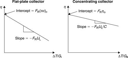
FIGURE 4.3 Typical collector performance curves.
A comparison of the efficiency of various collectors at irradiance levels of 500 and 1000 W/m2 is shown in Figure 4.4 (Kalogirou, 2004). Five representative collector types are considered:
• Advanced flat-plate collector (AFP). In this collector, the risers are ultrasonically welded to the absorbing plate, which is also electroplated with chromium selective coating.
• Stationary compound parabolic collector (CPC) oriented with its long axis in the east–west direction.
• Evacuated tube collector (ETC).
• Parabolic trough collector (PTC) with E–W tracking.
As seen in Figure 4.4, the higher the irradiation level, the better is the efficiency, and the higher performance collectors, such as the CPC, ETC, and PTC, retain high efficiency, even at higher collector inlet temperatures. It should be noted that the radiation levels examined are considered as global radiation for all collector types except the PTC, for which the same radiation values are used but considered as beam radiation.
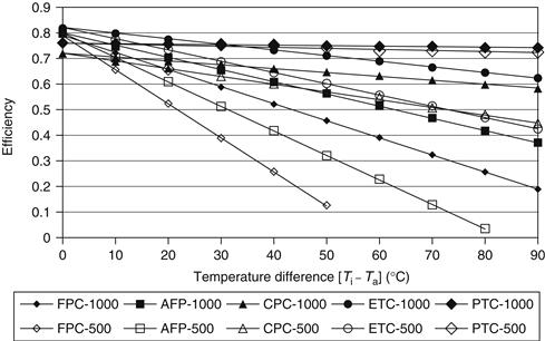
FIGURE 4.4 Comparison of the efficiency of various collectors at two irradiation levels: 500 and 1000 W/m2.
In reality, the heat loss coefficient, UL, in Eqs (4.3)–(4.6) is not constant but is a function of the collector inlet and ambient temperatures. Therefore,
![]() (4.8)
(4.8)
Applying Eq. (4.8) in Eqs (4.3) and (4.5), we have the following.
For flat-plate collectors:
![]() (4.9)
(4.9)
and for concentrating collectors:
![]() (4.10)
(4.10)
Therefore, for FPCs, the efficiency can be written as:
![]() (4.11)
(4.11)
and if we denote co = FR(τα)n and x = (Ti − Ta)/Gt, then:
![]() (4.12)
(4.12)
And, for concentrating collectors, the efficiency can be written as:
![]() (4.13)
(4.13)
and if we denote ko = FRηo, k1 = c1/C, k2 = c2/C, and y = (Ti − Ta)/GB, then:
![]() (4.14)
(4.14)
The difference in performance between flat-plate and concentrating collectors can also be seen from the performance equations. For example, the performance of a good FPC is given by:
![]() (4.15)
(4.15)
whereas the performance equation of the Industrial Solar Technologies (IST) PTC is:
![]() (4.16)
(4.16)
By comparing Eqs (4.15) and (4.16), we can see that FPCs usually have a higher intercept efficiency because their optical characteristics are better (no reflection losses), whereas the heat loss coefficients of the concentrating collectors are much smaller because these factors are inversely proportional to the concentration ratio.
In the above Equations ΔT or (Ti − Ta) is often termed reduced temperature difference. The standard ISO 9806-1:1994 allows the use of either (Ti − Ta) or (Tm − Ta), where Tm = (Ti + To)/2 is the mean temperature of the collector, whereas EN 12975-2:2006 only allows the latter. In this case the collector efficiency equation is modified as shown in Section 4.6.
Equations (4.11) and (4.13) include all important design and operational factors affecting steady-state performance, except collector flow rate and solar incidence angle. Flow rate inherently affects performance through the average absorber temperature. If the heat removal rate is reduced, the average absorber temperature increases and more heat is lost. If the flow is increased, collector absorber temperature and heat loss decrease. The effect of the solar incidence angle is accounted for by the incidence angle modifier, examined in Section 4.2.
4.1.1 Effect of flow rate
Experimental test data can be correlated to give values of FR(τα)n and FRUL for a particular flow rate used during the test. If the flow rate of the collector is changed from the test value during normal use, it is possible to calculate the new FR for the new flow rate using Eq. (3.58). A correction for the changed flow rate can be made if it is assumed that F′ does not change with flow rate, because of changes in hfi. The ratio r, by which the factors FR(τα)n and FRUL are corrected, is given by (Duffie and Beckman, 1991):
 (4.17a)
or
 (4.17b)
To use the above equations knowledge is required of the term F′UL. For the test conditions this can be calculated from Eq. (3.58) as the term FRUL is known from the performance testing. Therefore, by rearranging Eq. (3.58) we get:
![]() (4.18)
(4.18)
For liquid collectors F′UL is approximately equal for both test and use conditions, so the value estimated by Eq. (4.18) can be used in both cases in Eq. (4.17a).
For air collectors or for liquid collectors where hfi depends strongly on flow rate, F′ needs to be estimated for the new value of hfi using Eq. (3.48), (3.79) or (3.86a) according to the collector type. In this case hfi is estimated from the Nusselt number and the type of flow determined from the Reynolds number. For example for turbulent flow, the Nusselt number given by Eq. (3.131) can be used for internal pipe flows. For other cases appropriate equations can be used from heat transfer textbooks.
4.1.2 Collectors in series
Performance data for a single panel cannot be applied directly to a series of connected panels if the flow rate through the series is the same as for the single panel test data. If, however, N panels of the same type are connected in series and the flow is N times that of the single panel flow used during the testing, then the single panel performance data can be applied. If two panels are considered connected in series and the flow rate is set to a single panel test flow, the performance will be less than if the two panels were connected in parallel with the same flow rate through each collector. The useful energy output from the two collectors connected in series is then given by (Morrison, 2001):
![]() (4.19)
(4.19)
where To1 = outlet temperature from first collector given by:
![]() (4.20)
(4.20)
Eliminating To1 from Eqs (4.19) and (4.20) gives:
![]() (4.21)
(4.21)
where FR1, UL1, and (τα)1 are the factors for the single panel tested, and K is:
![]() (4.22)
(4.22)
For N identical collectors connected in series with the flow rate set to the single panel flow rate,
![]() (4.23)
(4.23)
![]() (4.24)
(4.24)
If the collectors are connected in series and the flow rate per unit aperture area in each series line of collectors is equal to the test flow rate per unit aperture area, then no penalty is associated with the flow rate other than an increased pressure drop from the circuit.
EXAMPLE 4.1
For five collectors in series, each 2 m2 in area and FR1UL1 = 4 W/m2 °C at a flow rate of 0.01 kg/s, estimate the correction factor. Water is circulated through the collectors.
Solution
From Eq. (4.22),
The factor
This example indicates that connecting collectors in series without increasing the working fluid flow rate in proportion to the number of collectors results in significant loss of output.
4.1.3 Standard requirements
Here, the various requirements of the ISO standards for both glazed and unglazed collectors are presented. For a more comprehensive list of the requirements and details on the test procedures, the reader is advised to read the actual standard.
Glazed collectors
To perform the steady-state test satisfactorily, according to ISO 9806-1:1994, certain environmental conditions are required (ISO, 1994):
1. Solar radiation greater than 800 W/m2.
2. Wind speed must be maintained between 2 and 4 m/s. If the natural wind is less than 2 m/s, an artificial wind generator must be used.
3. Angle of incidence of direct radiation is within ±2% of the normal incident angle.
4. Fluid flow rate should be set at 0.02 kg/s m2 and the fluid flow must be stable within ±1% during each test but may vary up to ±10% between different tests. Other flow rates may be used, if specified by the manufacturer.
5. To minimize measurement errors, a temperature rise of 1.5 K must be produced so that a point is valid.
Data points that satisfy these requirements must be obtained for a minimum of four fluid inlet temperatures, which are evenly spaced over the operating range of the collector. The first must be within ±3 K of the ambient temperature to accurately obtain the test intercept, and the last should be at the maximum collector operating temperature specified by the manufacturer. If water is the heat transfer fluid, 70 °C is usually adequate as a maximum temperature. At least four independent data points should be obtained for each fluid inlet temperature. If no continuous tracking is used, then an equal number of points should be taken before and after local solar noon for each inlet fluid temperature. Additionally, for each data point, a preconditioning period of at least 15 min is required, using the stated inlet fluid temperature. The actual measurement period should be four times greater than the fluid transit time through the collector with a minimum test period of 15 min.
To establish that steady-state conditions exist, average values of each parameter should be taken over successive periods of 30 s and compared with the mean value over the test period. A steady-state condition is defined as the period during which the operating conditions are within the values given in Table 4.1.
Table 4.1
Tolerance of Measured Parameters for Glazed Collectors
| Parameter | Deviation from the Mean |
| Total solar irradiance | ±50 W/m2 |
| Ambient air temperature | ±1 K |
| Wind speed | 2–4 m/s |
| Fluid mass flow rate | ±1% |
| Collector inlet fluid temperature | ±0.1 K |
Unglazed collectors
Unglazed collectors are more difficult to test, because their operation is influenced by not only the solar radiation and ambient temperature but also the wind speed. The last factor influences the collector performance to a great extent, since there is no glazing. Because it is very difficult to find periods of steady wind conditions (constant wind speed and direction), the ISO 9806-3:1995 for unglazed collector testing recommends that an artificial wind generator is used to control the wind speed parallel to the collector aperture (ISO, 1995b). The performance of unglazed collectors is also a function of the module size and may be influenced by the solar absorption properties of the surrounding ground (usually roof material), so to reproduce these effects a minimum module size of 5 m2 is recommended and the collector should be tested in a typical roof section. In addition to the measured parameters listed at the beginning of this chapter, the longwave thermal irradiance in the collector plane needs to be measured. Alternatively, the dew point temperature could be measured, from which the longwave irradiance may be estimated.
Similar requirements for preconditioning apply here as in the case of glazed collectors. However, the length of the steady-state test period in this case should be more than four times the ratio of the thermal capacity of the collector to the thermal capacity flow rate ![]() of the fluid flowing through the collector. In this case, the collector is considered to operate under steady-state conditions if, over the testing period, the measured parameters deviate from their mean values by less than the limits given in Table 4.2.
of the fluid flowing through the collector. In this case, the collector is considered to operate under steady-state conditions if, over the testing period, the measured parameters deviate from their mean values by less than the limits given in Table 4.2.
Table 4.2
Tolerance of Measured Parameters for Unglazed Collectors
| Parameter | Deviation from the Mean |
| Total solar irradiance | ±50 W/m2 |
| Longwave thermal irradiance | ±20 W/m2 |
| Ambient air temperature | ±1 K |
| Wind speed | ±0.25 m/s |
| Fluid mass flow rate | ±1% |
| Collector inlet fluid temperature | ±0.1 K |
Using a solar simulator
In countries with unsuitable weather conditions, the indoor testing of solar collectors with the use of a solar simulator is preferred. Solar simulators are generally of two types: those that use a point source of radiation mounted well away from the collector and those with large area multiple lamps mounted close to the collector. In both cases, special care should be taken to reproduce the spectral properties of the natural solar radiation. The simulator characteristics required are also specified in ISO 9806-1:1994 and the main ones are (ISO, 1994):
1. Mean irradiance over the collector aperture should not vary by more than ±50 W/m2 during the test period.
2. Radiation at any point on the collector aperture must not differ by more than ±15% from the mean radiation over the aperture.
3. The spectral distribution between wavelengths of 0.3 and 3 μm must be equivalent to air mass 1.5, as indicated in ISO 9845-1:1992.
4. Thermal irradiance should be less than 50 W/m2.
5. As in multiple lamp simulators, the spectral characteristics of the lamp array change with time, and as the lamps are replaced, the characteristics of the simulator must be determined on a regular basis.
Solar simulators can be divided into three main types: continuous, flash, and pulse. The first type is described above. This type is mostly used for low-intensity testing, varying from less than one to several suns.
The second type is the flash simulator. This is most suitable for testing photovoltaic (PV) cells and panels. The measurement with this solar simulator is instantaneous and lasts approximately as long as the flash of a camera (several milliseconds). Some models allow also the current–voltage (I–V) measurement of the PV. With this simulator very high intensities of up to several thousand suns are possible. The main advantage of this simulator is that it avoids heat buildup in the test specimen. The disadvantage is that due to the rapid heating and cooling of the lamp, the intensity and light spectrum are not constant, which may create reliability problems in repeated measurements.
The third type of solar simulator is the pulse simulator. This uses a shutter between the lamp and the specimen under test to quickly block or unblock the light. Pulses are typically of the order of 100 ms. In this case the lamp remains ON during the whole duration of the test and thus this simulator offers a compromise between the continuous and flash types. The disadvantages of this simulator are the high power consumption and the relatively low light intensities of the continuous type. The advantages are the stable light intensity and spectrum output and low thermal load imposed on the test specimen.
Leave a Reply