
The utilizability design concept is useful when the collector operates at a known critical radiation level during a specific month. In a practical system, however, the collector is connected to a storage tank, so the monthly sequence of weather and load time distributions cause a fluctuating storage tank temperature and thus a variable critical radiation level. On the other hand, the f-chart was developed to overcome the restriction of a constant critical level but is restricted to systems delivering a load near 20 °C.
Klein and Beckman (1979) combined the utilizability concept described in the previous section with the f-chart to produce the ![]() , f-chart design method for a closed loop solar energy system, shown in Figure 11.11. The method is not restricted to loads that are at 20 °C. In this system, the storage tank is assumed to be pressurized or filled with a liquid of high boiling point so that no energy dumping occurs through the relief valve. The auxiliary heater is in parallel with the solar energy system. In these systems, energy supplied to the load must be above a specified minimum useful temperature, Tmin, and it must be used at a constant thermal efficiency or coefficient of performance so that the load on the solar energy system can be estimated. The return temperature from the load is always at or above Tmin. Because the performance of a heat pump or a heat engine varies with the temperature level of supplied energy, this design method is not suitable for this kind of application. It is useful, however, in absorption refrigerators, industrial process heating, and space heating systems.
, f-chart design method for a closed loop solar energy system, shown in Figure 11.11. The method is not restricted to loads that are at 20 °C. In this system, the storage tank is assumed to be pressurized or filled with a liquid of high boiling point so that no energy dumping occurs through the relief valve. The auxiliary heater is in parallel with the solar energy system. In these systems, energy supplied to the load must be above a specified minimum useful temperature, Tmin, and it must be used at a constant thermal efficiency or coefficient of performance so that the load on the solar energy system can be estimated. The return temperature from the load is always at or above Tmin. Because the performance of a heat pump or a heat engine varies with the temperature level of supplied energy, this design method is not suitable for this kind of application. It is useful, however, in absorption refrigerators, industrial process heating, and space heating systems.
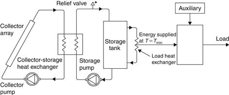
FIGURE 11.11 Schematic diagram of a closed-loop solar energy system.
The maximum monthly average daily energy that can be delivered from the system shown in Figure 11.11 is given by:
![]() (11.66)
(11.66)
This is the same as Eq. (11.65), except that ![]() is replaced with
is replaced with ![]() which is the maximum daily utilizability, estimated from the minimum monthly average critical radiation ratio:
which is the maximum daily utilizability, estimated from the minimum monthly average critical radiation ratio:
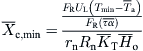 (11.67)
Klein and Beckman (1979) correlated the results of many detailed simulations of the system shown in Figure 11.11, for various storage size–collector-area ratios, with two dimensionless variables. These variables are similar to the ones used in the f-chart but are not the same. Here, the f-chart dimensionless parameter Y (plotted on the ordinate of the f-chart) is replaced by ![]() given by:
given by:
![]() (11.68)
(11.68)
And the f-chart dimensionless parameter X (plotted on the abscissa of the f-chart) is replaced by a modified dimensionless variable, X′, given by:
![]() (11.69)
(11.69)
In fact, the change in the X dimensionless variable is that the parameter ![]() is replaced with an empirical constant 100.
is replaced with an empirical constant 100.
The ![]() , f-charts can be obtained from actual charts or from the following analytical equation (Klein and Beckman, 1979):
, f-charts can be obtained from actual charts or from the following analytical equation (Klein and Beckman, 1979):
![]() (11.70)
(11.70)
where Rs = ratio of standard storage heat capacity per unit of collector area of 350 kJ/m2 °C to actual storage capacity, given by (Klein and Beckman, 1979):
![]() (11.71)
(11.71)
where M = actual mass of storage capacity (kg).
Although, in Eq. (11.70), f is included on both sides of equation, it is relatively easy to solve for f by trial and error. Since the ![]() , f-charts are given for various storage capacities and the user has to interpolate, the use of Eq. (11.70) is preferred, so the actual charts are not included in this book. The
, f-charts are given for various storage capacities and the user has to interpolate, the use of Eq. (11.70) is preferred, so the actual charts are not included in this book. The ![]() , f-charts are used in the same way as the f-charts. The values of
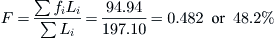
, f-charts are used in the same way as the f-charts. The values of ![]() Y, and X′ need to be calculated from the long-term radiation data for the particular location and load patterns. As before, fL is the average monthly contribution of the solar energy system, and the monthly values can be summed and divided by the total annual load to obtain the annual fraction, F.
Y, and X′ need to be calculated from the long-term radiation data for the particular location and load patterns. As before, fL is the average monthly contribution of the solar energy system, and the monthly values can be summed and divided by the total annual load to obtain the annual fraction, F.
EXAMPLE 11.13
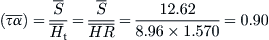
An industrial process heat system has a 50 m2 collector. The system is located at Nicosia, Cyprus (35°N latitude), and the collector characteristics are FRUL = 5.92 W/m2 °C, FR(τα)n = 0.82, tilted at 40°, and double glazed. The process requires heat at a rate of 15 kW at a temperature of 70 °C for 10 h each day. Estimate the monthly and annual solar fractions. Additional information is (τα)n = 0.96, storage volume = 5000 l. The weather conditions, as obtained from Appendix 7, are given in Table 11.13. The values of the last column are estimated from Eq. (2.82a).
Table 11.13
Weather Conditions for Example 11.13
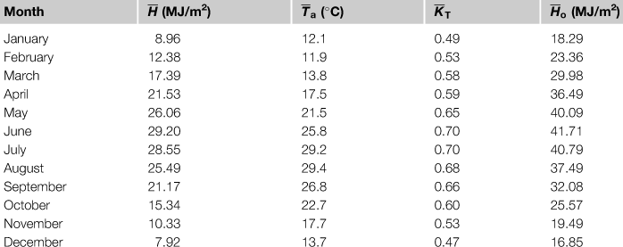
As can be seen, the values of ![]() are slightly different from those shown in Table 2.5 for 35°N latitude. This is because the actual latitude of Nicosia, Cyprus, is 35.15°N, as shown in Appendix 7.
are slightly different from those shown in Table 2.5 for 35°N latitude. This is because the actual latitude of Nicosia, Cyprus, is 35.15°N, as shown in Appendix 7.
Solution
To simplify the solution, most of the results are given directly in Table 11.14. These concern ![]() given by Eq. (2.108);
given by Eq. (2.108); ![]() given by Eqs (2.105c) and (2.105d);
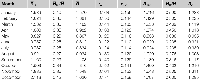
given by Eqs (2.105c) and (2.105d); ![]() given by Eq. (2.107); rn and rd,n, given by Eqs (2.84) and (2.83), respectively, at noon (h = 0°); RB,n, given by Eq. (2.90a) at noon; HD/H, given by Eqs (11.54); and Rn, given by Eq. (11.53).
given by Eq. (2.107); rn and rd,n, given by Eqs (2.84) and (2.83), respectively, at noon (h = 0°); RB,n, given by Eq. (2.90a) at noon; HD/H, given by Eqs (11.54); and Rn, given by Eq. (11.53).
Table 11.14
Results of Radiation Coefficients for Example 11.13
Subsequently, the data for January are presented. First, we need to estimate ![]() . For this estimation, we need to know
. For this estimation, we need to know ![]() and then apply Eq. (11.10) to find the required parameter. From Eqs (3.4a) and (3.4b),
and then apply Eq. (11.10) to find the required parameter. From Eqs (3.4a) and (3.4b),


From Figure 3.27, for a double-glazed collector,
and
Therefore,


These values are constant for all months. For the beam radiation, we use Figures A3.8(a) and A3.8(b) to find the equivalent angle for each month and Figure 3.27 to get (τα)/(τα)n. The 12 angles are 40, 42, 44, 47, 50, 51, 51, 49, 46, 43, 40, and 40, from which 12 values are read from Figure 3.27 and the corresponding values are given in Table 11.15. The calculations for January are as follows:
From the data presented in previous tables,
From Eq. (2.106),

and
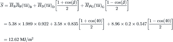
From Eq. (11.10),
The results for the other months are shown in Table 11.15.
Table 11.15
Results of ![]() for Other Months for Example 11.13
for Other Months for Example 11.13
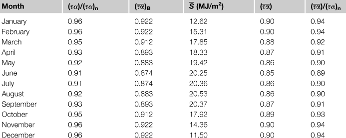
Now we can proceed with the ![]() f-chart method calculations. Again, the estimations for January are shown in detail below. The minimum monthly average critical radiation ratio is given by Eq. (11.67):
f-chart method calculations. Again, the estimations for January are shown in detail below. The minimum monthly average critical radiation ratio is given by Eq. (11.67):
From Eq. (11.56),


The load for January is:

From Eq. (11.68),

From Eq. (11.69),

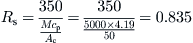
The storage parameter, Rs, is estimated with Eq. (11.71):
Finally, f can be calculated from Eq. (11.70). The solar contribution is fL. The calculations for the other months are shown in Table 11.16. The use of a spreadsheet program greatly facilitates calculations.
Table 11.16
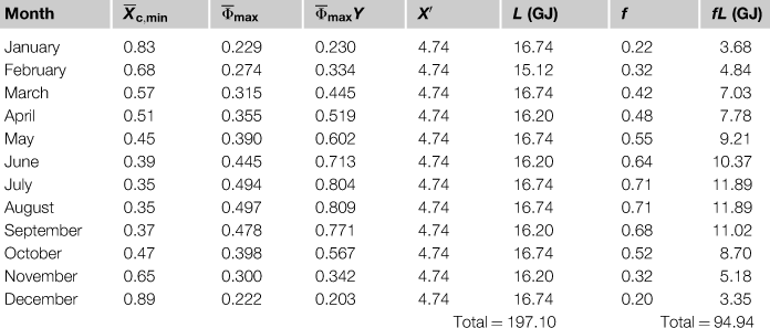
The annual fraction is given by Eq. (11.12):
It should be pointed out that the ![]() f-chart method overestimates the monthly solar fraction, f. This is due to assumptions that there are no losses from the storage tank and that the heat exchanger is 100% efficient. These assumptions require certain corrections, which follow.
f-chart method overestimates the monthly solar fraction, f. This is due to assumptions that there are no losses from the storage tank and that the heat exchanger is 100% efficient. These assumptions require certain corrections, which follow.
11.3.1 Storage tank-losses correction
The rate of energy lost from the storage tank to the environment, which is at temperature Tenv, is given by:
![]() (11.72)
(11.72)
The storage tank losses for the month can be obtained by integrating Eq. (11.72), considering that (UA)s and Tenv are constant for the month:
![]() (11.73)
(11.73)
where ![]() = monthly average storage tank temperature (°C).
= monthly average storage tank temperature (°C).
Therefore, the total load on the solar energy system is the actual load required by a process and the storage tank losses. Because the storage tanks are usually well insulted, storage tank losses are small and the tank rarely drops below the minimum temperature. The fraction of the total load supplied by the solar energy system, including storage tank losses, is given by:
Leave a Reply