Frequency Modulation and Demodulation

With frequency modulation the frequency (rather than the amplitude) of a constant-amplitude, constant-frequency sinusoidal carrier is made to vary in proportion to the amplitude of the applied modulating signal. This is shown in Figure 19.10, where a constant-amplitude carrier is frequency-modulated by a single tone. Note how the frequency of the carrier changes.

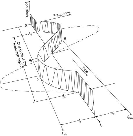
Figure 19.10 Constant-amplitude carrier is frequency-modulated by single tone

Frequency modulation can be understood by considering Figure 19.11. This shows that a modulating square or sine wave may be used for this type of modulation. The frequency of the frequency-modulated carrier remains constant, and this indicates that the modulating process does not increase the power of the carrier wave. For FM the instantaneous frequency ω is made to vary as

(19.10)

In this equation

(19.11)

And we have:

(19.12)

Substituting (19.12) into (19.11) gives:

(19.13)

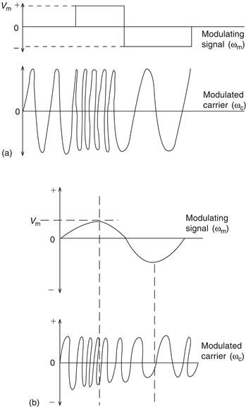
Figure 19.11 Use of modulating square or sine wave in frequency modulation

for the peak angular frequency shift for the modulating signal.

The modulating index is given by:

(19.14)

for a constant frequency, constant amplitude modulating signal. In practice the modulating signal varies in amplitude and frequency. This leads to two further parameters: a maximum value of the modulating signal (f_m(max)); and a maximum allowable frequency shift, which is defined as the frequency deviation (f_d). The deviation ratio (δ) is then defined as:

(19.15)

For any given FM system the frequency will swing to a maximum value of frequency deviation known as the rated system derivation. This parameter determines the maximum allowable modulating signal voltage. Equation (19.15) applies for this condition of rated system deviation.

Finally, the frequency-modulated wave can be written as:

(19.16)

for a constant-amplitude, constant-frequency modulating signal such as a square wave, and,

(19.17)

for a variable-amplitude, variable-frequency modulating signal such as a sinusoidal wave.

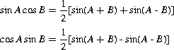
Expanding (19.17) using the identity:

gives,

The second factor of each term expands into an infinite series whose coefficients are a function of δ. These coefficients are called Bessel functions, denoted by J_n(δ), which vary as δ varies. More specifically, they are Bessel functions of the first kind and of order n.

Expanding the second factor gives

and,

Using the relationships:

we obtain:

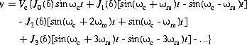
Thus the modulated wave consists of a carrier and an infinite number of upper and lower side-frequencies spaced at intervals equal to the modulation frequency. Also, since the amplitude of the unmodulated and modulated waves are the same, the powers in the unmodulated and modulated waves are equal.

The Bessel coefficients can be determined either from graphs or tables.

Example 19.5

Determine the values of the amplitudes of the carrier and side frequencies if f_d is 5 kHz, f_m(max) is 5 kHz and the carrier amplitude is 10 V.

Solution

The deviation ratio is unity and the sideband amplitudes and carrier amplitude are:

As the carrier has an amplitude of 10 V, each component in the spectrum diagram will have the values shown in Figure 19.12.

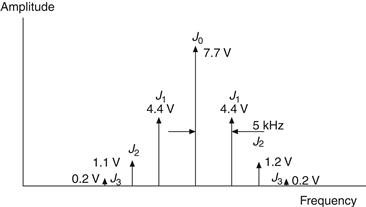
Figure 19.12 Spectrum diagram for Example 19.5

Example 19.6

Determine the amplitudes of the side frequencies generated by an FM transmitter having a deviation ratio of 10 kHz, a modulating frequency of 5 kHz and a carrier level of 10 V.

Solution

The deviation ratio is 2 for this system, so once again the following amplitudes are obtained.

The spectrum diagram is shown in Figure 19.13. There are more side frequencies in this case and hence, the quality of the transmission would be improved. However, not all the side frequencies are relevant, as can be seen from their amplitudes.

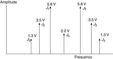
Figure 19.13 Spectrum diagram for Example 19.6

19.4.1 Bandwidth and Carson’s Rule

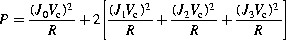
It has already been mentioned that not all the side frequencies are necessary for satisfactory performance. Generally, an acceptable performance can be obtained with a finite number of side frequencies, and this may be considered satisfactory when not less than 98% of the power is contained in the carrier and its adjacent frequencies. Since the amplitude of the nth side frequency is given as J_nV_c, the power dissipated in a load (R) by the modulated wave is:

(19.18)

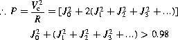
Thus, for 98% of the power to be contained in the carrier plus the side frequencies, the following applies:

Example 19.7

An FM transmitter transmits with a rated system deviation of 60 kHz and a maximum modulating frequency of 15 kHz. If the carrier amplitude is 25 V, determine the number of side frequencies required to ensure that 98% of the power is contained in the carrier and side frequencies. Sketch the spectrum diagram.

Solution

The frequency deviation is given by:

From the Bessel tables,

It will be seen that only J₂, J₃, J₄, J₅ and J₀ are required:

The spectrum diagram is sketched in Figure 19.14.

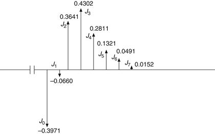
Figure 19.14 Spectrum diagram for Example 19.7

The Bessel tables show negative and positive values for the Bessel functions J₀, J₁, J₂ etc. When the deviation ratio is zero, the carrier is unmodulated and has its maximum value. For any other modulation index the energy levels are distributed between the sidebands and carrier. As the deviation ratio increases the number of sidebands increases, as does the number of negative values. The negative values indicate a 180° phase shift, and this can be seen from the Bessel graphs where the carrier and each sideband behave as sinusoids as frequency deviation takes place. Negative signs are usually ignored in practice, since only the magnitude of the carrier and each sideband is required. Squaring the negative values produces positive or magnitude quantities.

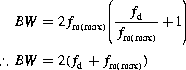
Example 19.7 shows that not all of the side frequencies are necessary for a high-fidelity output in an FM system. The bandwidth can therefore be determined by considering only the useful side frequencies with the higher amplitudes. Note that the required bandwidth, when all the side frequencies are considered, is given as

This is a considerable saving in bandwidth and hence a reduction in noise in the modulator circuits.

For a rated system deviation the required bandwidth for Example 19.7 is:

Also since δ=4,

This indicates the required number of pairs of side frequencies for the 98% criterion.

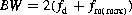
Since BW=(δ+1) pairs of side frequencies, i.e.,

(19.19)

Since,

substituting in (19.19) gives:

(19.20)

Equations (19.19) and (19.20) express a relationship known as Carson’s rule for determining the bandwidth of an FM system requiring the requisite number of side frequencies to satisfy the 98% criterion. Also δ indicates the rated system deviation, while β is used for values less than this.

Example 19.8

(a) An FM system uses a carrier frequency of 100 MHz with an amplitude of 100 V. It is modulated by a 10 kHz signal and the rated system deviation is 80 kHz. Determine the amplitude of the center frequency.

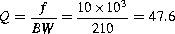
(b) An FM station with a maximum modulating frequency of 15 kHz and a deviation ratio of 6 operates at a center frequency (f_c) of 10 MHz. Determine the 3 dB bandwidth of the stage following the modulator which would pass 98% of the power in the modulated wave. Also determine the Q factor of this circuit.

Solution

(a) 

For δ=8, the Bessel tables give J₀=0.1717. Therefore the amplitude of the center frequency is:

(b) Assume rated system deviation. Thus:

Also, 

Hence, 

so,

Example 19.9

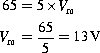
An FM system has a rated system deviation of 65 kHz. Determine the maximum permitted value of the modulating signal voltage if the modulator has a sensitivity of 5 kHz/V.

Solution

Since the maximum swing is 65 kHz, then:

Example 19.10

An FM broadcast station is assigned a channel between 92.1 and 92.34 MHz. If the maximum modulating frequency is 15 kHz determine:

(a) the maximum permissible value of the deviation ratio;

(b) the number of side frequencies.

Solution

(a) 

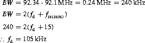
Also, 

(b) From the Bessel tables, this will give 10 pairs of sidebands.