R–L SERIES CIRCUIT

A circuit that contains a pure resistance R Ω connected in series with a coil having pure inductance of L Henry is known as R–L series circuit. This is the most general case that we come across in practice.

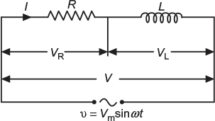
Fig. 7.7  Circuit containing resistance and inductance in series

An R–L series circuit and its phasor diagram are shown in Figures 7.7 and 7.8, respectively. To draw the phasor diagram, current I (rms value) is taken as the reference vector. Voltage drop in resistance V_R (=IR) is taken in phase with current vector, whereas voltage drop in inductive reactance V_L (=IX_L) is taken 90° ahead of the current vector (since current lags behind the voltage by 90° in pure inductive circuit). The vector sum of these two voltages (drops) is equal to the applied voltage V (rms value).

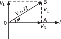
Fig. 7.8  Phasor diagram

Now, V_R = IR and V_L = IX_L (where X_L = 2 π f L)

In right−angled triangle OAB,

or

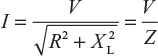
where  is the total opposition offered to the flow of AC by an R–L series circuit and is called impedance of the circuit. It is measured in ohms.

7.6.1  Phase Angle

From the phasor diagram shown in Figure 7.8, it is clear that current in this circuit lags behind the applied voltage by an angle ɸ called phase angle.

From phasor diagram, 

7.6.2  Power

If the alternating voltage applied across the circuit is given by the equation.

 

ν = V_m sin ω t

Then,

 

i = I_m sin (ω t − ɸ )

∴Instantaneous power, p = vi

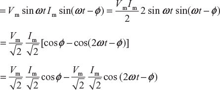
Average power consumed in the circuit over a complete cycle,

or

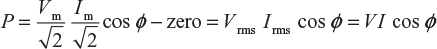
where cos ɸ is called power factor of the circuit.

From phasor diagram, 

Therefore, power factor is defined as the cosine of the angle between the voltage and the current in an AC circuit. It may also be defined as the ratio of resistance to impedance of an AC circuit.

Alternatively, power, 

This shows that power is actually consumed in resistance only; inductance does not consume any power.

7.6.3  Power Curve

The phasor diagram and wave diagram for voltage and current are shown in Figure 7.9(a) and (b), respectively, where applied voltage (v = V_m sin ω t) is taken as reference quantity. The power curve for R–L series circuit is also shown in Figure 7.9(b). The points on the power curve are obtained from the product of the corresponding instantaneous values of voltage and current. It is clear that power is negative between angle 0 and ɸ and between 180° and (180 + ɸ). During rest of the cycle, the power is positive. Since the area under the positive loops is greater than that under the negative loops, the net power over a complete cycle is positive. Hence, a definite quantity of power is utilised or consumed by this circuit.

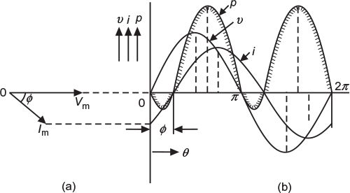
Fig. 7.9  (a) Phasor diagram (b) Wave diagram for voltage, current and power