
The following are examples of closed-loop control systems to illustrate how, despite the different forms of control being exercised, the systems all have the same basic structural elements.
18.7.1 Control of the Speed of Rotation of a Motor Shaft
Consider the motor system shown in Figure 18.61 for the control of the speed of rotation of the motor shaft and its block diagram representation in Figure 18.62. The input of the required speed value is by means of the setting of the position of the movable contact of the potentiometer. This determines what voltage is supplied to the comparison element, i.e., the differential amplifier, as indicative of the required speed of rotation. The differential amplifier produces an amplified output which is proportional to the difference between its two inputs. When there is no difference then the output is zero. The differential amplifier is thus used to both compare and implement the control law. The resulting control signal is then fed to a motor which adjusts the speed of the rotating shaft according to the size of the control signal. The speed of the rotating shaft is measured using a tachogenerator, this being connected to the rotating shaft by means of a pair of bevel gears. The signal from the tachogenerator gives the feedback signal which is then fed back to the differential amplifier.
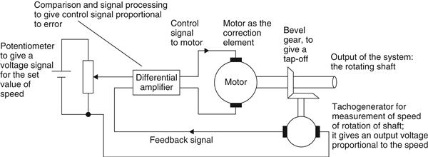
Figure 18.61 Control of the speed of rotation of a shaft
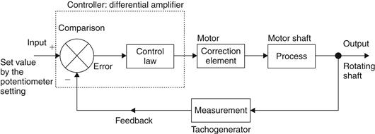
Figure 18.62 Control of the speed of rotation of a shaft
18.7.2 Control of the Position of a Tool
Figure 18.63 shows a position control system using a belt driven by a stepper motor to control the position of a tool and Figure 18.64 its block diagram representation. The inputs to the controller are the required position voltage and a voltage giving a measure of the position of the workpiece, this being provided by a potentiometer being used as a position sensor. Because a microprocessor is used as the controller, these signals have to be processed to be digital. The output from the controller is an electrical signal which depends on the error between the required and actual positions and is used, via a drive unit, to operate a stepper motor. Input to the stepper motor causes it to rotate its shaft in steps, so rotating the belt and moving the tool.
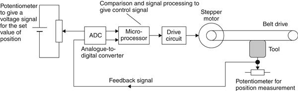
Figure 18.63 Position control system
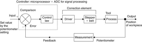
Figure 18.64 Position control system
18.7.3 Power Steering
Control systems are used to not only maintain some variable constant at a required value but also to control a variable so that it follows the changes required by a variable input signal. An example of such a control system is the power steering system used with a car. This comes into operation whenever the resistance to turning the steering wheel exceeds a predetermined amount and enables the movement of the wheels to follow the dictates of the angular motion of the steering wheel. The input to the system is the angular position of the steering wheel. This mechanical signal is scaled down by gearing and has subtracted from it a feedback signal representing the actual position of the wheels. This feedback is via a mechanical linkage. Thus when the steering wheel is rotated and there is a difference between its position and the required position of the wheels, there is an error signal. The error signal is used to operate a hydraulic valve and so provide a hydraulic signal to operate a cylinder. The output from the cylinder is then used, via a linkage, to change the position of the wheels. Figure 18.65 shows a block diagram of the system.
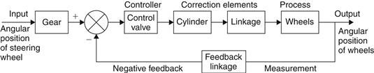
Figure 18.65 Power assisted steering
18.7.4 Control of Fuel Pressure
The modem car involves many control systems. For example, there is the engine management system aimed at controlling the amount of fuel injected into each cylinder and the time at which to fire the spark for ignition. Part of such a system is concerned with delivering a constant pressure of fuel to the ignition system. Figure 18.66(a) shows the elements involved in such a system. The fuel from the fuel tank is pumped through a filter to the injectors, the pressure in the fuel line being controlled to be 2.5 bar (2.5×0.1 MPa) above the manifold pressure by a regulator valve. Figure 18.66(b) shows the principles of such a valve. It consists of a diaphragm which presses a ball plug into the flow path of the fuel. The diaphragm has the fuel pressure acting on one side of it and on the other side is the manifold pressure and a spring. If the pressure is too high, the diaphragm moves and opens up the return path to the fuel tank for the excess fuel, so adjusting the fuel pressure to bring it back to the required value.
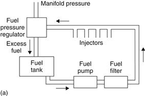
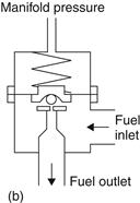
Figure 18.66 (a) Fuel supply system; (b) fuel pressure regulator
The pressure control system can be considered to be represented by the closed loop system shown in Figure 18.67. The set value for the pressure is determined by the spring tension. The comparator and control law is given by the diaphragm and spring. The correction element is the ball in its seating and the measurement is given by the diaphragm.
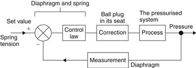
Figure 18.67 Fuel supply control system
18.7.5 Antilock Brakes
Another example of a control system used with a car is the antilock brake system (ABS). If one or more of the vehicle’s wheels lock, i.e., begins to skid, during braking, then braking distance increases, steering control is lost and tire wear increases. Antilock brakes are designed to eliminate such locking. The system is essentially a control system which adjusts the pressure applied to the brakes so that locking does not occur. This requires continuous monitoring of the wheels and adjustments to the pressure to ensure that, under the conditions prevailing, locking does not occur. Figure 18.68 shows the principles of such a system.
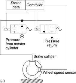
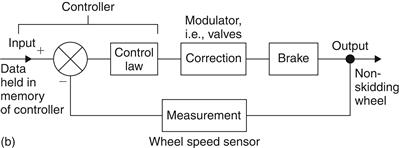
Figure 18.68 Antilock brakes: (a) schematic diagram;(b) block form of the control system
The two valves used to control the pressure are solenoid-operated valves, generally both valves being combined in a component termed the modulator. When the driver presses the brake pedal, a piston moves in a master cylinder and pressurises the hydraulic fluid. This pressure causes the brake calliper to operate and the brakes to be applied. The speed of the wheel is monitored by means of a sensor. When the wheel locks, its speed changes abruptly and so the feedback signal from the sensor changes. This feedback signal is fed into the controller where it is compared with what signal might be expected on the basis of data stored in the controller memory. The controller can then supply output signals which operate the valves and so adjust the pressure applied to the brake.
18.7.6 Thickness Control
As an illustration of a process control system, Figure 18.69 shows the type of system that might be used to control the thickness of sheet produced by rollers, Figure 18.70 showing the block diagram description of the system. The thickness of the sheet is monitored by a sensor such as a linear variable differential transformer (LVDT). The position of the LVDT probe is set so that when the required thickness sheet is produced, there is no output from the LVDT. The LVDT produces an alternating current output, the amplitude of which is proportional to the error. This is then converted to a DC error signal which is fed to an amplifier. The amplified signal is then used to control the speed of a DC motor, generally being used to vary the armature current. The rotation of the shaft of the motor is likely to be geared down and then used to rotate a screw which alters the position of the upper roll, hence changing the thickness of the sheet produced.
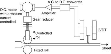
Figure 18.69 Sheet thickness control system
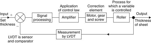
Figure 18.70 Sheet thickness control system
18.7.7 Control of Liquid Level
Figure 18.71 shows a control system used to control the level of liquid in a tank using a float-operated pneumatic controller, Figure 18.72 showing a block diagram of the system. When the level of the liquid in the tank is at the required level and the inflow and outflows are equal, then the controller valves are both closed. If there is a decrease in the outflow of liquid from the tank, the level rises and so the float rises. This causes point P to move upward. When this happens, the valve connected to the air supply opens and the air pressure in the system increases. This causes a downward movement of the diaphragm in the flow control valve and hence, a downward movement of the valve stem and the valve plug. This then results in the inflow of liquid into the tank being reduced. The increase in the air pressure in the controller chamber causes the bellows to become compressed and move that end of the linkage downward. This eventually closes off the valve so that the flow control valve is held at the new pressure and hence the new flow rate.
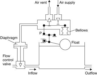
Figure 18.71 Level control system
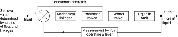
Figure 18.72 Level control system
If there is an increase in the outflow of liquid from the tank, the level falls and so the float falls. This causes point P to move downward. When this happens, the valve connected to the vent opens and the air pressure in the system decreases. This causes an upward movement of the diaphragm in the flow control valve and hence an upward movement of the valve stem and the valve plug. This then results in the inflow of liquid into the tank being increased. The bellows react to this new air pressure by moving its end of the linkage, eventually closing off the exhaust and so holding the air pressure at the new value and the flow control valve at its new flow rate setting.
18.7.8 Robot Gripper
The term robot is used for a machine which is a reprogrammable multi-function manipulator designed to move tools, parts, materials, etc. through variable programmed motions in order to carry out specified tasks. Here just one aspect will be considered, the gripper used by a robot at the end of its arm to grip objects. A common form of gripper is a device which has “fingers” or “jaws.” The gripping action then involves these clamping on the object. Figure 18.73 shows one form such a gripper can take if two gripper fingers are to close on a parallel sided object. When the input rod moves toward the fingers they pivot about their pivots and move closer together. When the rod moves outward, the fingers move further apart. Such motion needs to be controlled so that the grip exerted by the fingers on an object is just sufficient to grip it, too little grip and the object will fall out of the grasp of the gripper and too great might result in the object being crushed or otherwise deformed. Thus there needs to be feedback of the forces involved at contact between the gripper and the object. Figure 18.74 shows the type of closed-loop control system involved.
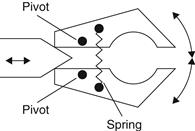
Figure 18.73 An example of a gripper
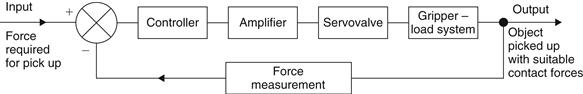
Figure 18.74 Gripper control system
The drive system used to operate the gripper can be electrical, pneumatic or hydraulic. Pneumatic drives are very widely used for grippers because they are cheap to install, the system is easily maintained and the air supply is easily linked to the gripper. Where larger loads are involved, hydraulic drives can be used. Sensors that might be used for measurement of the forces involved are piezoelectric sensors or strain gauges. Thus when strain gauges are stuck to the surface of the gripper and forces applied to a gripper, the strain gauges will be subject to strain and give a resistance change related to the forces experienced by the gripper when in contact with the object being picked up.
The robot arm with gripper is also likely to have further control loops to indicate when it is in the fight position to grip an object. Thus the gripper might have a control loop to indicate when it is in contact with the object being picked up; the gripper can then be actuated and the force control system can come into operation to control the grasp. The sensor used for such a control loop might be a microswitch which is actuated by a lever, roller or probe coming into contact with the object.
18.7.9 Machine Tool Control
Machine tool control systems are used to control the position of a tool or workpiece and the operation of the tool during a machining operation. Figure 18.75 shows a block diagram of the basic elements of a closed-loop system involving the continuous monitoring of the movement and position of the work tables on which tools are mounted while the workpiece is being machined. The amount and direction of movement required in order to produce the required size and form of workpiece is the input to the system, this being a program of instructions fed into a memory which then supplies the information as required. The sequence of steps involved is then:
1. An input signal is fed from the memory store.
2. The error between this input and the actual movement and position of the work table is the error signal which is used to apply the correction. This may be an electric motor to control the movement of the work table. The work table then moves to reduce the error so that the actual position equals the required position.
3. The next input signal is fed from the memory store.
5. The next input signal is fed from the memory store, and so on.
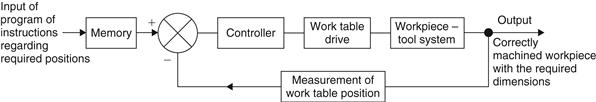
Figure 18.75 Closed-loop machine tool control system
18.7.10 An Automatic Drill
As an illustration of the type of control that might be used with a machine consider the system for a drill which is required to automatically drill a hole in a workpiece when it is placed on the work table (Figure 18.76). A switch sensor can be used to detect when the workpiece is on the work table. This then gives an on input signal to the controller and it then gives an output signal to actuate a motor to lower the drill head and commence drilling. When the drill reaches the full extent of its movement in the workpiece, the drill head triggers another switch sensor. This provides an on input to the controller and it then reverses the direction of rotation of the drill head motor and the drill retracts. This is an example of closed-loop discrete-event control.
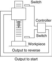
Figure 18.76 An automatic drill
18.7.11 Microprocessor-Controlled Systems
The control system used in many modem consumer products, e.g., in a modem motor car or a modem washing machine, to exercise control is likely to be a microprocessor-based system. The controller is then basically as shown in Figure 18.77. It compares the input from a sensor with what is required and then, using a control law determined by the program stored in its memory, gives an output to a correction element.
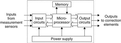
Figure 18.77 Microprocessor-based controller
Leave a Reply