
The following describes how we can arrive at the input-output relationships for systems by representing them by simple models obtained by considering them to be composed of just a few simple basic elements.
18.10.1 Mechanical Systems
Mechanical systems, however complex, have stiffness (or springiness), damping and inertia and can be considered to be composed of basic elements which can be represented by springs, dashpots and masses.
The “springiness” or “stiffness” of a system can be represented by a spring. For a linear spring (Figure 18.84(a)), the extension y is proportional to the applied extending force F and we have:

where k is a constant termed the stiffness.
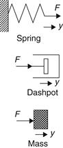
Figure 18.84 Mechanical system building blocks
The “damping” of a mechanical system can be represented by a dashpot. This is a piston moving in a viscous medium in a cylinder (Figure 18.84(b)). Movement of the piston inward requires the trapped fluid to flow out past edges of the piston; movement outward requires fluid to flow past the piston and into the enclosed space. The resistive force F which has to be overcome is proportional to the velocity of the piston and hence the rate of change of displacement y with time, i.e., dy/dt. Thus:

where c is a constant.
The “inertia” of a system—i.e., how much it resists being accelerated—can be represented by mass. For a mass m (Figure 18.84(c)), the relationship between the applied force F and its acceleration a is given by Newton’s second law as F=ma. But acceleration is the rate of change of velocity v with time t, i.e., a=dv/dt, and velocity is the rate of change of displacement y with time, i.e., v=dy/dt. Thus a=d(dy/dt)/dt and so we can write:

The following example illustrates how we can arrive at a model for a mechanical system.
Example 18.5
Derive a model for the mechanical system given in Figure 18.85(a). The input to the system is the force F and the output is the displacement y.
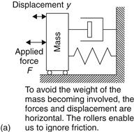
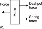
Figure 18.85 (a) Mechanical system with mass, damping and stiffness; (b) the free-body diagram for the forces acting on the mass
Solution
To obtain the system model we draw free-body diagrams, these being diagrams of masses showing just the external forces acting on each mass. For the system in Figure 18.84(a) we have just one mass and so just one free-body diagram and that is shown in Figure 18.84(b). As the free-body diagram indicates, the net force acting on the mass is the applied force minus the forces exerted by the spring and by the dashpot:
net force =![]()
Then applying Newton’s second law, this force must be equal to ma, where a is the acceleration, and so:
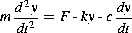
The relationship between the input F to the system and the output y is described by the second-order differential equation:
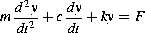
The term second-order is used because the equation includes as its highest derivative d2y/dt2.
18.10.2 Rotational Systems
For rotational systems the basic building blocks are a torsion spring, a rotary damper and the moment of inertia (Figure 18.86).
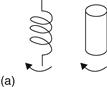


Figure 18.86 Rotational system elements: (a) torsional spring or elastic twisting of a shaft; (b) rotational dashpot; (c) moment of inertia
The “springiness” or “stiffness” of a rotational spring is represented by a torsional spring. For a torsional spring, the angle θ rotated is proportional to the torque T:

where k is a measure of the stiffness of the spring.
The damping inherent in rotational motion is represented by a rotational dashpot. For a rotational dashpot, i.e., effectively a disk rotating in a fluid, the resistive torque T is proportional to the angular velocity ω and thus:

where c is the damping constant.
The inertia of a rotational system is represented by the moment of inertia of a mass. A torque T applied to a mass with a moment of inertia I results in an angular acceleration a and thus, since angular acceleration is the rate of change of angular velocity ω with time, i.e., dω/dt, and angular velocity ω is the rate of change of angle with time, i.e., dθ/dt, then the angular acceleration is d(dθ/dt)/dt and so:

The following example illustrates how we can arrive at a model for a rotational system.
Example 18.6
Develop a model for the system shown in Figure 18.87(a) of the rotation of a disk as a result of twisting a shaft.
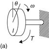
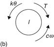
Figure 18.87 Example
Solution
Figure 18.87(b) shows the free-body diagram for the system. The torques acting on the disk are the applied torque T, the spring torque kθ and the damping torque cω. Hence:
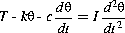
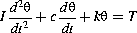
We thus have the second-order differential equation relating the input of the torque to the output of the angle of twist:
18.10.3 Electrical Systems
The basic elements of electrical systems are the resistor, inductor and capacitor (Figure 18.88).
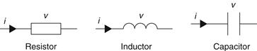
Figure 18.88 Electrical system building blocks
For a resistor, resistance R, the potential difference v across it when there is a current i through it is given by:

For an inductor, inductance L, the potential difference v across it at any instant depends on the rate of change of current i and is:

For a capacitor, the potential difference v across it depends on the charge q on the capacitor plates with v=q/C, where C is the capacitance. Thus:


Since current i is the rate of movement of charge:
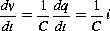
and so we can write:

To develop the models for electrical circuits we use Kirchhoff’s laws. These can be stated as:
The total current flowing into any circuit junction is equal to the total current leaving that junction, i.e., the algebraic sum of the currents at a junction is zero.
In a closed circuit path, termed a loop, the algebraic sum of the voltages across the elements that make up the loop is zero. This is the same as saying that for a loop containing a source of e.m.f., the sum of the potential drops across each circuit element is equal to the sum of the applied e.m.f.’s, provided we take account of their directions.
The following examples illustrate the development of models for electrical systems.
Example 18.7
Develop a model for the electrical system described by the circuit shown in Figure 18.89. The input is the voltage v when the switch is closed and the output is the voltage vc across the capacitor.
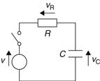
Figure 18.89 Electrical system with resistance and capacitance
Solution
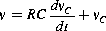
Using Kirchhoff’s voltage law gives:

and, since VR=Ri and i=C(dvc/dt) we obtain the equation:
The relationship between an input v and the output vc is a first order differential equation. The term first-order is used because it includes as its highest derivative dvC/dt.
Example 18.8
Develop a model for the circuit shown in Figure 18.90 when we have an input voltage v when the switch is closed and take an output as the voltage vc across the capacitor.
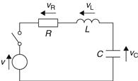
Figure 18.90 Electrical system with resistance, inductance and capacitance
Solution
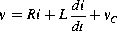
Applying Kirchhoff’s voltage law gives:

and so:
Since i=C(dvC/dt), then di/dt=C(d2vC/dt2) and thus, we can write:
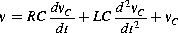
The relationship between an input v and output vc is described by a second-order differential equation.
18.10.4 Thermal Systems
Thermal systems have two basic building blocks, resistance and capacitance (Figure 18.91).
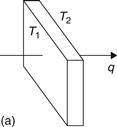
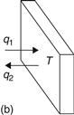
Figure 18.91 (a) Thermal resistance; (b) thermal capacitance
The thermal resistance R is the resistance offered to the rate of flow of heat q (Figure 18.91(a)) and is defined by:

where T1– is the temperature difference through which the heat flows.
For heat conduction through a solid we have the rate of flow of heat proportional to the cross-sectional area and the temperature gradient. Thus for two points at temperatures T1 and T2 and a distance L apart:

with k being the thermal conductivity. Thus with this mode of heat transfer, the thermal resistance R is L/Ak. For heat transfer by convection between two points, Newton’s law of cooling gives:

where (T2–T1) is the temperature difference, h the coefficient of heat transfer and A the surface area across which the temperature difference is. The thermal resistance with this mode of heat transfer is thus 1/Ah.
The thermal capacitance (Figure 18.91(b)) is a measure of the store of internal energy in a system. If the rate of flow of heat into a system is q1, and the rate of flow out q2 then the rate of change of internal energy of the system is q1-q2. An increase in internal energy can result in a change in temperature:

where m is the mass and c the specific heat capacity. Thus the rate of change of internal energy is equal to mc times the rate of change of temperature. Hence:
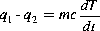
This equation can be written as:

where the capacitance C=mc.
The following example illustrates the development of models for thermal systems.
Example 18.9
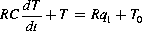
Develop a model for the simple thermal system of a thermometer at temperature T being used to measure the temperature of a liquid when it suddenly changes to the higher temperature of TL (Figure 18.92).
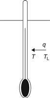
Figure 18.92 Example
Solution
When the temperature changes there is heat flow q from the liquid to the thermometer. The thermal resistance to heat flow from the liquid to the thermometer is:

Since there is only a net flow of heat from the liquid to the thermometer the thermal capacitance of the thermometer is:

Substituting for q gives:

which, when rearranged gives:
This is a first-order differential equation.
Example 18.10
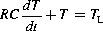
Determine a model for the temperature of a room (Figure 18.93) containing a heater which supplies heat at the rate q1 and the room loses heat at the rate q2.
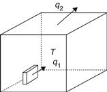
Figure 18.93 Example
Solution
We will assume that the air in the room is at a uniform temperature T. If the air and furniture in the room have a combined thermal capacity C, since the energy rate to heat the room is q1–q2, we have:

If the temperature inside the room is T and that outside the room T0 then

where R is the thermal resistance of the walls. Substituting for q2 gives:
Hence:
This is a first-order differential equation.
18.10.5 Hydraulic Systems
For a fluid system the three building blocks are resistance, capacitance and inertance; these are the equivalents of electrical resistance, capacitance and inductance. The equivalent of electrical current is the volumetric rate of flow and of potential difference is pressure difference. Hydraulic fluid systems are assumed to involve an incompressible liquid; pneumatic systems, however, involve compressible gases and consequently there will be density changes when the pressure changes. Here we will just consider the simpler case of hydraulic systems. Figure 18.94 shows the basic form of building blocks for hydraulic systems.
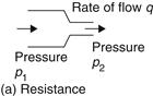
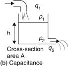
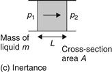
Figure 18.94 Hydraulic building blocks
Hydraulic resistance R is the resistance to flow which occurs when a liquid flows from one diameter pipe to another (Figure 18.94(a)) and is defined as being given by the hydraulic equivalent of Ohm’s law:

Hydraulic capacitance C is the term used to describe energy storage where the hydraulic liquid is stored in the form of potential energy (Figure 18.94(b)). The rate of change of volume V of liquid stored is equal to the difference between the volumetric rate at which liquid enters the container q1 and the rate at which it leaves q2, i.e.,

But V=Ah and so:

The pressure difference between the input and output is:

Hence, substituting for h gives:

The hydraulic capacitance C is defined as:

and thus, we can write:

Hydraulic inertance is the equivalent of inductance in electrical systems. To accelerate a fluid a net force is required and this is provided by the pressure difference (Figure 18.93(c)). Thus:
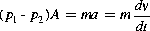
where a is the acceleration and so the rate of change of velocity v. The mass of fluid being accelerated is m=ALp and the rate of flow q=Av and so:
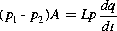

where the inertance I is given by I=Lp/A.
The following example illustrates the development of a model for a hydraulic system.
Example 18.11
Develop a model for the hydraulic system shown in Figure 18.95 where there is a liquid entering a container at one rate q1 and leaving through a valve at another rate q2.
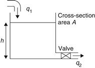
Figure 18.95 Example
Solution
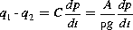
We can neglect the inertance since flow rates can be assumed to change only very slowly. For the capacitance term we have:
For the resistance of the valve we have:

Thus, substituting for q2, and recognizing that the pressure difference is hpg, gives:
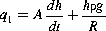
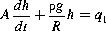
This is a first-order differential equation.
Leave a Reply