
The following are examples of sensors that are commonly used with the measurement systems of control systems.
18.4.1 Potentiometer
A potentiometer consists of a resistance element with a sliding contact which can be moved over the length of the element and connected as shown in Figure 18.13. With a constant supply voltage Vs the output voltage Vo between terminals 1 and 2 is a fraction of the input voltage, the fraction depending on the ratio of the resistance R12 between terminals 1 and 2 compared with the total resistance R of the entire length of the track across which the supply voltage is connected. Thus Vo/Vs=R12/R. If the track has a constant resistance per unit length, the output is proportional to the displacement of the slider from position 1. A rotary potentiometer consists of a coil of wire wrapped round into a circular track or a circular film of conductive plastic over which a rotatable sliding contact can be rotated, hence an angular displacement can be converted into a potential difference. Linear tracks can be used for linear displacements.
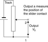
Figure 18.13 Potentiometer as a sensor of position
18.4.2 Strain-Gauged Element
Figure 18.14(a) shows the basic form of an electrical resistance strain gauge. Strain gauges consist of a fiat length of metal wire, metal foil strip, or a strip of semiconductor material which can be stuck onto surfaces like a postage stamp. When the wire, foil, strip or semiconductor is stretched, its resistance R changes. The fractional change in resistance —R/R is proportional to the strain ε, i.e.:

where G, the constant of proportionality, is termed the gauge factor. Metal strain gauges typically have gauge factors of the order of 2.0.
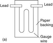
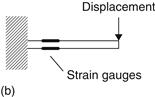
Figure 18.14 (a) Strain gauge; (b) example of use on a cantilever to provide a displacement sensor
When such a strain gauge is stretched, its resistance increases, when compressed its resistance decreases. A displacement sensor might be constructed by attaching strain gauges to a cantilever (Figure 18.14(b)), the free end of the cantilever being moved as a result of the linear displacement being monitored. When the cantilever is bent, the electrical resistance strain gauges mounted on the element are strained and so give a resistance change which can be monitored and which is a measure of the displacement. With strain gauges mounted as shown in Figure 18.14, when the cantilever is deflected downward the gauge on the upper surface is stretched and the gauge on the lower surface compressed. Thus the gauge on the upper surface increases in resistance while that on the lower surface decreases.
18.4.3 Linear Variable Differential Transformer
The linear variable differential transformer, generally referred to by the abbreviation LVDT, is a transformer with a primary coil and two secondary coils. Figure 18.15 shows the arrangement, there being three coils symmetrically spaced along an insulated tube. The central coil is the primary coil and the other two are identical secondary coils which are connected in series in such a way that their outputs oppose each other. A magnetic core is moved through the central tube as a result of the displacement being monitored. When there is an alternating voltage input to the primary coil, alternating e.m.f.s are induced in the secondary coils. With the magnetic core in a central position, the amount of magnetic material in each of the secondary coils is the same and so the e.m.f.s induced in each coil are the same. Since they are so connected that their outputs oppose each other, the net result is zero output. However, when the core is displaced from the central position there is a greater amount of magnetic core in one coil than the other. The result is that a greater e.m.f. is induced in one coil than the other and then there is a net output from the two coils. The bigger the displacement the more of the core there is in one coil than the other, thus the difference between the two e.m.f.s increases the greater the displacement of the core. Typically, LVDTs have operating ranges from about ±2 mm to ±400 mm and are very widely used for monitoring displacements.
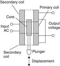
Figure 18.15 LVDT: Giving an output voltage related to the position of the plunger
18.4.4 Optical Encoders
An encoder is a device that provides a digital output as a result of an angular or linear displacement. Position encoders can be grouped into two categories: incremental encoders, which detect changes in displacement from some datum position, and absolute encoders, which give the actual position.
Figure 18.16 shows the basic form of an incremental encoder for the measurement of angular displacement of a shaft. It consists of a disc which rotates along with the shaft. In the form shown, the rotatable disc has a number of windows through which a beam of light can pass and be detected by a suitable light sensor. When the shaft and disc rotates, a pulsed output is produced by the sensor with the number of pulses being proportional to the angle through which the disc rotates. The angular displacement of the disc, and hence the shaft rotating it, can thus be determined by the number of pulses produced in the angular displacement from some datum position. Typically the number of windows on the disc varies from 60 to over a thousand with multi-tracks having slightly offset slots in each track. With 60 slots occurring with 1 revolution then, since 1 revolution is a rotation of 360° the minimum angular displacement, i.e., the resolution, that can be detected is 360/60=6°. The resolution typically varies from about 6° to 0.3° or better.
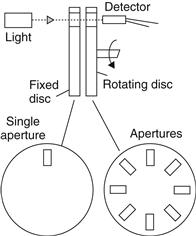
Figure 18.16 Incremental encoder: angular displacement results in pulses being detected, the number of pulses being proportional to the angular displacement
With the incremental encoder, the number of pulses counted gives the angular displacement, a displacement of, say, 50° giving the same number of pulses whatever angular position the shaft starts its rotation from. However, the absolute encoder gives an output in the form of a binary number of several digits, each such number representing a particular angular position. Figure 18.17 shows the basic form of an absolute encoder for the measurement of angular position. With the one shown in the figure, the rotating disc has four concentric circles of slots and four sensors to detect the light pulses. The slots are arranged in such a way that the sequential output from the sensors is a number in the binary code, each such number corresponding to a particular angular position. A number of forms of binary code are used. Typical encoders tend to have up to 10 or 12 tracks. The number of bits in the binary number will be equal to the number of tracks. Thus with 10 tracks there will be 10 bits and so the number of positions that can be detected is 210, i.e., 1024, a resolution of 360/1024=0.35°.
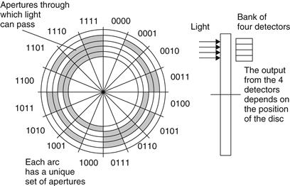
Figure 18.17 The rotating wheel of the absolute encoder: the binary word output indicates the angular position
18.4.5 Switches
There are many situations where a sensor is required to detect the presence of some object. The sensor used in such situations can be a mechanical switch, giving an on-off output when the switch contacts are opened or closed by the presence of an object. Figure 18.18 illustrates the forms of a number of such switches. An example of switch application is where a work piece closes the switch by pushing against it when it reaches the correct position on a work table, such a switch being referred to as a limit switch. The switch might then be used to switch on a machine tool to carry out some operation on the work piece.
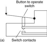
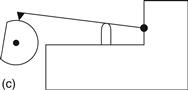
Figure 18.18 Limit switches: (a) Lever; (b) roller; (c) cam
18.4.6 Tachogenerator
The basic tachogenerator consists of a coil mounted in a magnetic field (Figure 18.19). When the coil rotates electromagnetic induction results in an alternating e.m.f. being induced in the coil. The faster the coil rotates the greater the size of the alternating e.m.f. Thus the size of the alternating e.m.f. is a measure of the angular speed.
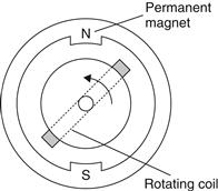
Figure 18.19 The tachogenerator
18.4.7 Pressure Sensors
The movement of the center of a circular diaphragm as a result of a pressure difference between its two sides is the basis of a pressure gauge (Figure 18.20(a)). For the measurement of the absolute pressure, the opposite side of the diaphragm is a vacuum, for the measurement of pressure difference the pressures are connected to each side of the diaphragm, for the gauge pressure, i.e., the pressure relative to the atmospheric pressure, the opposite side of the diaphragm is open to the atmosphere. The amount of movement with a plane diaphragm is fairly limited; greater movement can, however, be produced with a diaphragm with corrugations (Figure 18.20(b)).
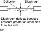
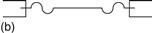
Figure 18.20 Diaphragm sensors
The movement of the center of a diaphragm can be monitored by some form of displacement sensor. Figure 18.21 shows the form that might be taken when strain gauges are used to monitor the displacement, the strain gauges being stuck to the diaphragm and changing resistance as a result of the diaphragm movement. Typically such sensors are used for pressures over the range 100 kPa to 100 MPa, with an accuracy up to about ±0.1%. Another form of diaphragm pressure gauge uses strain gauge elements integrated within a silicon diaphragm and supplied, together with a resistive network for signal processing, on a single silicon chip as the Motorola MPX pressure sensor. With a voltage supply connected to the sensor, it gives an output voltage directly proportional to the pressure. Such sensors are available for use for the measurement of absolute pressure, differential pressure or gauge pressure; for example, MPX2100 has a pressure range of 100 kPa and with a supply voltage of 16V DC gives a voltage output over the full range of 40 mV.
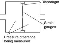
Figure 18.21 Pressure gauge with strain gauges to sense movement of the diaphragm
When certain crystals are stretched or compressed, charges appear on their surfaces. This effect is called piezo-electricity. Examples of such crystals are quartz, tourmaline, and zirconate-titanate. A piezoelectric pressure gauge consists essentially of a diaphragm which presses against a piezoelectric crystal (Figure 18.22). Movement of the diaphragm causes the crystal to be compressed and so charges produced on its surface. The crystal can be considered to be a capacitor which becomes charged as a result of the diaphragm movement and so a potential difference appears across it. If the pressure keeps the diaphragm at a particular displacement, the resulting electrical charge is not maintained but leaks away. Thus the sensor is not suitable for static pressure measurements. Typically, such a sensor can be used for pressures up to about 1000 MPa.
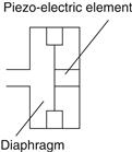
Figure 18.22 Basic form of a piezo-electric sensor
18.4.8 Fluid Flow
The traditional methods used for the measurement of fluid flow involve devices based on Bernoulli’s equation. When a restriction occurs in the path of a flowing fluid, a pressure drop is produced with the flow rate being proportional to the square root of the pressure drop. Hence, a measurement of the pressure difference can be used to give a measure of the rate of flow. There are many devices based on this principle. The Venturi tube is a tube which gradually tapers from the full pipe diameter to the constricted diameter. Figure 18.23 shows the typical form of such a tube. The pressure difference is measured between the flow prior to the constriction and at the constriction, a diaphragm pressure cell generally being used. The orifice plate (Figure 18.24) is simply a disc, with generally a central hole. The orifice plate is placed in the tube through which the fluid is flowing and the pressure difference measured between a point equal to the diameter of the tube upstream and a point equal to half the diameter downstream. Because of the way the fluid flows through the orifice plate, such measurements are equivalent to those taken with the Venturi tube.
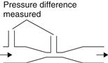
Figure 18.23 Venturi tube: pressure difference is a measure of the flow rate
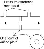
Figure 18.24 Orifice plate
The turbine flowmeter (Figure 18.25) consists of a multi-bladed rotor that is supported centrally in the pipe along which the flow occurs. The rotor rotates as a result of the fluid flow, the angular velocity being approximately proportional to the flow rate. The rate of revolution of the rotor can be determined by attaching a small permanent magnet to one of the blades and using a pick-up coil. An induced e.m.f, pulse is produced in the coil every time the magnet passes it. The pulses are counted and so the number of revolutions of the rotor can be determined. The meter is expensive, with an accuracy of typically about ±0.1%.
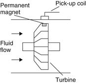
Figure 18.25 Basic principle of the turbine flowmeter: number of pulses picked-up per second is a measure of flow rate
18.4.9 Liquid Level
A commonly used method to measure the level of liquid in a vessel is a float whose position is directly related to the liquid level. Figure 18.26 shows a simple float system. The float is at one end of a pivoted rod with the other end connected to the slider of a potentiometer. Changes in level cause the float to move and hence move the slider over the potentiometer resistance track and so give a potential difference output related to the liquid level.
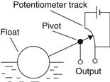
Figure 18.26 Potentiometer float gauge: as the float rises the output voltage decreases
18.4.10 Temperature Sensors
The expansion or contraction of solids, liquids or gases, the change in electrical resistance of conductors and semiconductors, thermoelectric e.m.f.s and the change in the current across the junction of semiconductor diodes and transistors are all examples of properties that change when the temperature changes and can be used as basis of temperature sensors.
The bimetallic strip device consists of two different metal strips of the same length bonded together (Figure 18.27). Because the metals have different coefficients of expansion, when the temperature increases the composite strip bends into a curved strip, with the higher coefficient metal on the outside of the curve. The amount by which the strip curves depends on the two metals used, the length of the composite strip and the change in temperature. If one end of a bimetallic strip is fixed, the amount by which the free end moves is a measure of the temperature. This movement may be used to open or close electric circuits, as in the simple thermostat commonly used with domestic heating systems. Bimetallic strip devices are robust, relatively cheap, have an accuracy of the order of ±1% and are fairly slow reacting to changes in temperature.
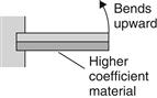
Figure 18.27 Bimetallic strip; as the temperature increases it bends upward with the higher coefficient material extending more than the lower coefficient material
Resistance temperature detectors (RTDs) are simple resistive elements in the form of coils of wire of such metals as platinum, nickel or copper alloys, the resistance varying as the temperature changes with the change in resistance being reasonably proportional to the change in temperature. Detectors using platinum have high linearity, good repeatability, high long term stability, can give an accuracy of ±0.5% or better, a range of about -200°C to +850°C can be used in a wide range of environments without deterioration, but are more expensive than the other metals. They are, however, very widely used. Nickel and copper alloys are cheaper but have less stability, are more prone to interaction with the environment and cannot be used over such large temperature ranges.
Thermistors are semiconductor temperature sensors made from mixtures of metal oxides, such as those of chromium, cobalt, iron, manganese and nickel. The resistance of thermistors decreases in a very nonlinear manner with an increase in temperature, Figure 18.28 illustrating this. The change in resistance per degree change in temperature is considerably larger than that which occurs with metals. For example, a thermistor might have a resistance of 29 kΩ at -20°C, 9.8 kΩ at 0°C, 3.75 kΩ at 20°C, 1.6 kΩ at 40°C, 0.75 kΩ at 60°C. The material is formed into various forms of element, such as beads, discs and rods (Figure 18.29). Thermistors are rugged and can be very small, so enabling temperatures to be monitored at virtually a point. Because of their small size they have small thermal capacity and so respond very rapidly to changes in temperature. The temperature range over which they can be used will depend on the thermistor concerned, ranges within about -100°C to +300°C being possible. They give very large changes in resistance per degree change in temperature and so are capable, over a small range, of being calibrated to give an accuracy of the order of 0.1°C or better. However, their characteristics tend to drift with time. Their main disadvantage is their nonlinearity.
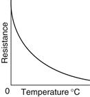
Figure 18.28 Variation of resistance with temperature for thermistors


Figure 18.29 Thermistors: (a) rod; (b) disc; (c) bead
When two different metals are joined together, a potential difference occurs across the junction. The potential difference depends on the two metals used and the temperature of the junction. A thermocouple involves two such junctions, as illustrated in Figure 18.30. If both junctions are at the same temperature, the potential differences across the two junctions cancel each other out and there is no net e.m.f. If, however, there is a difference in temperature between the two junctions, there is an e.m.f. The value of this e.m.f. E depends on the two metals concerned and the temperatures t of both junctions. Usually one junction is held at 0°C and then, to a reasonable extent, the following relationship holds:

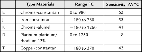
where a and b are constants for the metals concerned. Figure 18.31 shows how the e.m.f, varies with temperature for a number of commonly used pairs of metals. Standard tables giving the e.m.f.s at different temperatures are available for the metals usually used for thermocouples. Commonly used thermocouples are listed in Table 18.1, with the temperature ranges over which they are generally used and typical sensitivities. These commonly used thermocouples are given reference letters. The base-metal thermocouples, E, J, K and T, have accuracies about ±1 to 3%, are relatively cheap but deteriorate with age. Noblemetal thermocouples, e.g., R have accuracies of about ±1% or better, are more expensive but more stable with longer life. Thermocouples are generally mounted in a sheath to give them mechanical and chemical protection. The response time of an unsheathed thermocouple is very fast. With a sheath this may be increased to as much as a few seconds if a large sheath is used.
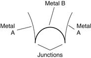
Figure 18.30 Thermocouple: a temperature difference between the junctions gives a voltage between them
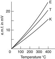
Figure 18.31 Thermocouples: chromel-constantan (E), chromelalumel (K), copper-constantan (T)
Table 18.1
Thermocouples
To maintain one junction of a thermocouple at 0°C it needs to be immersed in a mixture of ice and water. This, however, is often not convenient. A compensation circuit (Figure 18.32) can, however, be used to provide an e.m.f. which varies with the temperature of the cold junction in such a way that when it is added to the thermocouple e.m.f. it generates a combined e.m.f. which is the same as would have been generated if the cold junction had been at 0°C.
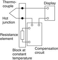
Figure 18.32 Cold junction compensation to compensate for the cold junction not being at 0°C
There is a change in the current across the junction of semiconductor diodes and transistors when the temperature changes. For use as temperature sensors they are supplied, together with the necessary signal processing circuitry, as integrated circuits. An integrated circuit temperature sensor using transistors is LM35. This gives an output, which is a linear function of temperature, of 10 mV/°C when the supply voltage is 5 V. Figure 18.33(a) shows the connections for the range 12°C to 110°C and (b) for -40°C to 110°C.
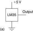
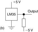
Figure 18.33 LM35 connections
Leave a Reply