
As has already been mentioned, the higher the order of filter the sharper the cut-off. For certain applications, such as radio relay applications and channel separation, it is necessary to have higher-order filters. This chapter only looks at first and second-order filters but many higher orders can be designed by simply cascading these two types; indeed, this is one of the big advantages of using the active filter.
17.6.1 Low-Pass Second-Order Filters
Consider two low-pass first-order filters with the same cut-off frequencies, but different pass-band gains:
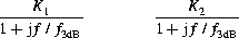
If these filters are now cascaded, then the overall function will appear as follows,
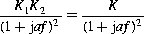
where a=1/f3dB and K=K1K2.
Expanding the above expression will give:
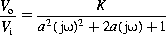
and in general terms this is stated as:
![]() (17.7)
(17.7)
where a1 and a2 are constants. This expression is the characteristic of a second-order filter, and from it two basic types of filter may be deduced, depending on the values of a1 and a2: Butterworth flat response, where ![]() ; and Chebyshev ripple response, where
; and Chebyshev ripple response, where ![]() . The responses of both these filters has already been given, but they are combined in Figure 17.14.
. The responses of both these filters has already been given, but they are combined in Figure 17.14.
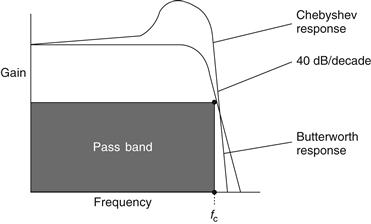
Figure 17.14 Responses for both low-pass second-order filters
The Butterworth response is generally a flatter response than the Chebyshev, but the Chebyshev filter has a faster rate of cut-off immediately after the cut-off frequency. Because of its flat response the Butterworth filter is more popular, but the ripple response of the Chebyshev has applications in satellite transponders where channel separation is tight.
Both these filters can be represented by many circuits, but the easiest configuration is known as the Sallen-Key circuit from which most filters may be designed, provided the pass-band gain and cut-off frequency are known. The typical circuit configuration is shown in Figure 17.15.
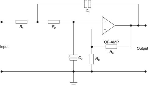
Figure 17.15 Sallen-Key circuit
By using circuit analysis the general transfer function for the circuit in Figure 17.15 may be determined as follows:
![]() (17.8)
(17.8)
where K=1+Ra/Rb (the DC gain) and s=jω. A full analysis of the transfer function can be found in standard texts on filters.
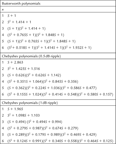
The denominator term in equation (17.7) is known as the polynomial for the nth-order filter. These polynomials may be derived for any filter type or order, but it is more convenient to use polynomial tables. Examples given in this text will use polynomials which are shown in Table 17.1.
Table 17.1
Filter polynomials
This form of the general transfer function is related to Figure 17.15 where R1, C1, etc. are the components used in the Sallen-Key circuit after a multiplication factor has been applied. This is called denormalization.
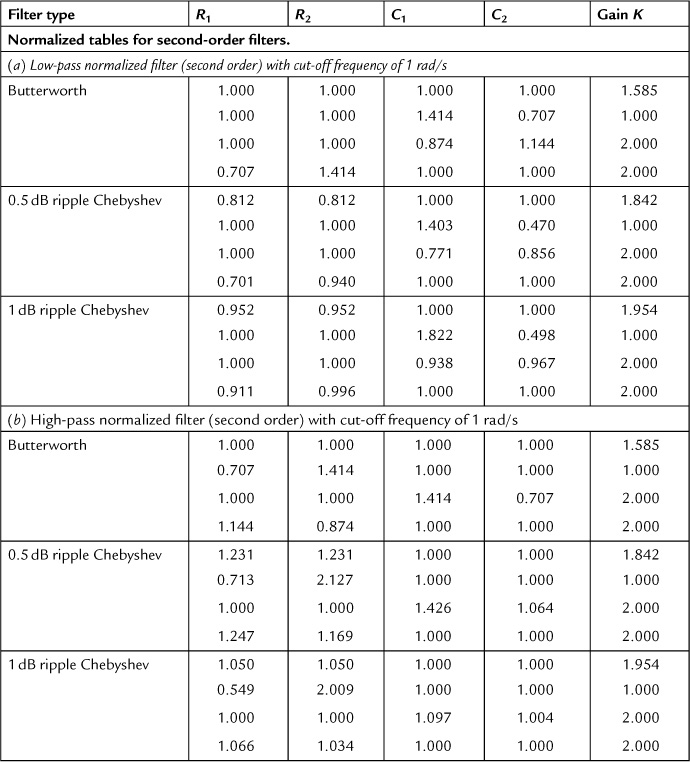
Later in this chapter normalized filter tables, given in Table 17.2, will be used. The term normalization is defined usually as the scaling or standardization of a certain parameter. In the case of the filter tables the values are normalized to an angular cut-off frequency of 1 rad/s or 1 Hz. A multiplier is used in order to calculate the actual values of the components which will be used in the printed circuit board design. The operation of this multiplier is known as denormalization and will be fully demonstrated by the examples given later.
Table 17.2
Normalized filter tables
It is as well to appreciate at this point that filter problems may be solved by using four main methods: the transfer function; normalized tables; identical components; and software. The use of software is widespread and there are many software packages which can be easily used by the novice. The suitability of these packages is a personal matter, but the author has found that the use of spreadsheets gives excellent results. The other three methods of solving active filter problems will be demonstrated by example
Leave a Reply