Second-Order High-Pass Filters

High-pass filters may be designed in a similar manner to low-pass second-order filters, but in this case the normalized response is slightly different. The response for such a filter may be given as:

(17.18)

As before two cases are deduced: the Chebyshev response, where  an the Butterworth response, where . These responses are shown in Figure 17.18.

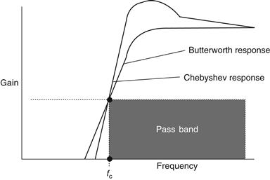
Figure 17.18 Responses for second-order high-pass filters

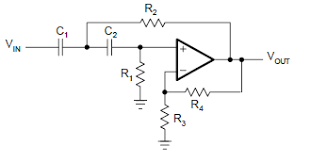
As before, a Sallen-Key circuit can be drawn, and this is almost identical to the low-pass circuit except that the components are interchanged. Such a circuit is shown in Figure 17.19.

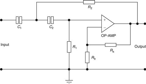
Figure 17.19 Sallen-Key circuit for high-pass filter

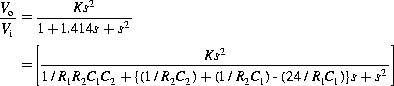
The transfer function is the same as for the low-pass filter, but it should be remembered that the components have been interchanged and because of this it will now take the form:

(17.19)

which is in the form:

Problems are tackled in exactly the same way as for the low-pass case, and normalized tables may be used in a similar fashion. The following worked examples will now clarify the principles discussed so far.

Example 17.7

Draw the circuit of a first-order low-pass Butterworth filter having a cut-off frequency of 10 kHz and a pass-band gain of unity.

Solution

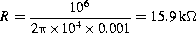
Choose a value C=0.001 μF. Hence,

The circuit for this solution is shown in Figure 17.20.

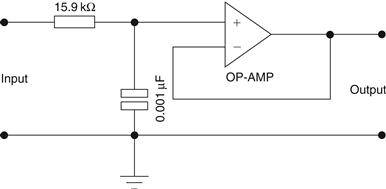
Figure 17.20 Circuit for Example 17.7

Example 17.8

Figure 17.21 represents a first-order filter. Draw the response for this filter showing scaling and relevant points.

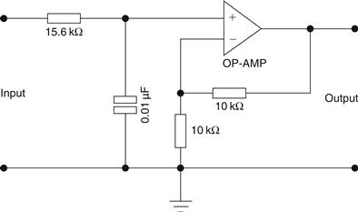
Figure 17.21 First-order filter for Example 17.8

Solution

Gain is given by:

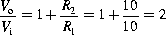
Since R=15.6 kΩ and C=0.01 μF,

The response for this problem is shown in Figure 17.22.

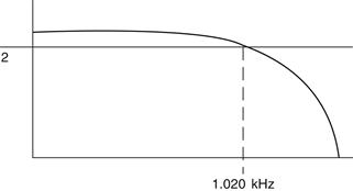
Figure 17.22 Response for Example 17.8

Example 17.9

Design a -40 dB/decade low pass filter at a cut-off frequency of 10 krad/s, assuming equal value components.

Solution

As equal value components are used, from the normalized tables the gain must be 1.585. Hence, as the angular frequency is 10 krad/s,

and selecting a value for R at random, say 36 kΩ, then we simply apply this to the formula as follows:

The circuit is shown in Figure 17.23.

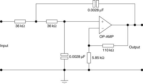
Figure 17.23 Circuit for Example 17.9

Example 17.10

Design a second-order high-pass filter which has a Butterworth response with a pass-band gain of 25 and a 3 dB cut-off frequency of 20 kHz. Note the second-order Butterworth coefficients are a₂=1 and a₁=1.414.

Solution

This type of problem unfortunately cannot be solved by the normalized tables; hence, the analytical method will be used.

The second-order Butterworth response is given by:

Equating as usual gives:

(17.20)

(17.21)

Let,

Therefore, from (17.20),

Hence, substituting in (17.21) gives,

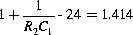
i.e.,

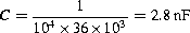
Letting C₁=1 F gives R₂=1/24.414=0.0410 Ω; thus C₂=24.414 F. Also C₁=1/R₁, therefore R₁=1 Ω. Assuming a denormalizing factor of 104, we have:

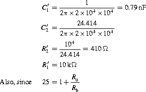
we have R_a=1 kΩ and R_b=24 kΩ. The circuit is shown in Figure 17.24.

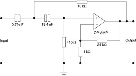
Figure 17.24 Circuit for Example 17.10

Example 17.11

Show how a third-order low-pass filter may be designed using a first- and second-order combination in order to achieve a pass-band gain of 2 and a cut-off frequency of 5 kHz.

Solution

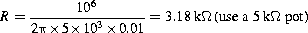
For the first-order stage we have:

Choosing a value for C=0.01 μF,

For the second-order stage the normalized tables are used for a pass-band gain of 2. Select R₁=R₂=1, C₁=0.874 and C₂=1.414. Using a denormalizing factor of 10⁴ gives the following values:

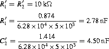
R_a/R_b=1, hence, let R_a=R_b=10 kΩ. The circuit is shown in Figure 17.25.

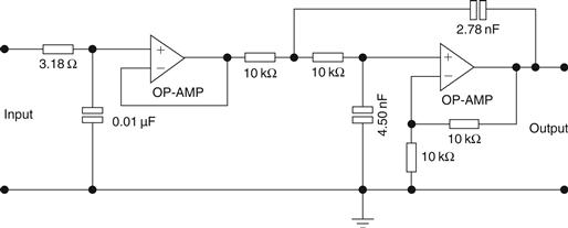
Figure 17.25 Circuit for Example 17.11