
Suppose we have a control system for the temperature in a room. How will the temperature react when the thermostat has its set value increased from, say, 20°C to 22°C? In order to determine how the output of a control system will react to different inputs, we need a mathematical model of the system so that we have an equation describing how the output of the system is related to its input.
Thus, in the case of an amplifier system (Figure 18.78) we might be able to use the simple relationship that the output is always 10 times the input. If we have an input of a 1 V signal we can calculate that the output will be 10V. This is a simple model of a system where the input is just multiplied by a gain of 10 in order to give the output.
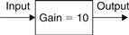
Figure 18.78 Amplifier system with the output ten times the input
However, if we consider a system representing a spring balance with an input of a load signal and an output of a deflection (Figure 18.79) then, when we have an input to the system and put a fixed load on the balance (this type of input is known as a step input because the input variation with time looks like a step), it is likely that it will not instantaneously give the weight but the pointer on the spring balance will oscillate for a little time before settling down to the weight value. Thus, we cannot just state, for an input of some constant load, that the output is just the input multiplied by some constant number but need some way of describing an output which varies with time. With an electrical system of a circuit with capacitance and resistance, when the voltage to such a circuit is switched on, i.e., there is a constant voltage input to the system, then the current changes with time before eventually settling down to a steady value. With a temperature control system, such as that used for the central heating system for a house, when the thermostat is changed from 20°C to 22°C the output does not immediately become 22°C but there is a change with time and eventually it may become 22°C In general, the mathematical model describing the relationship between input and output for a system is likely to involve terms which give values which change with time and are described by a differential equation (see Appendix B). As we continue through this chapter, we look at how such differential equation relationships arise.
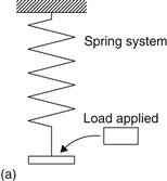
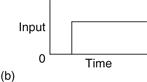
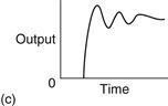
Figure 18.79 (a) The spring system with a constant load applied at some instant of time; (b) the step showing how the input varies with time; (c) the output showing how it varies with time for the step input
In order to make life simple, what we need is a simple relationship between input and output for a system, even when the output varies with time. It is nice and simple to say that the output is just ten times the input and so describe the system by gain =10. There is a way we can have such a simple form of relationship where the relationship involves time but it involves writing inputs and outputs in a different form. It is called the Laplace transform and it was covered earlier in Chapter 8. Let us consider how we can carry out such transformations; the aim is to enable you to use the transform as a tool to carry out tasks.
Leave a Reply