Clustering Techniques

Clustering is a set of techniques used to partition data into a number of groups, also called clusters. A cluster can be considered as a group of data objects that are similar to other objects in the same cluster and dis-similar to data objects in other clusters. Clustering helps data scientists to identify two main qualities of data—meaningfulness and usefulness.

Meaningful clusters enhance domain knowledge. For example, in the healthcare industry, clustering is used to make groups of patients whose bodies responded differently to the same medical treatment.

Useful clusters serve as an intermediate step in a data pipeline. For example, businesses use this technique for making different clusters of customers depending on their purchasing patterns to create targeted advertising campaigns.

2.5.1 Overview of Clustering Techniques

Data objects can be clustered using a variety of techniques. Each of these techniques has its own strengths and weaknesses. Depending upon the input data, we need to select the most appropriate technique that result in more natural cluster assignment. To select the most suitable clustering algorithm for the dataset is not a trivial task. Some important factors that affect this decision include the characteristics of the clusters, the features of the dataset, the number of outliers, and the number of data objects. Based on these features, three popular categories of clustering algorithms include:

1. Partitional clustering
2. Hierarchical clustering
3. Density-based clustering

Partitional Clustering

It divides data objects into non-overlapping groups in such a way that every object belongs to one and only one cluster, and every cluster must have at least one object.

In such algorithms, users can specify the number of clusters (indicated by the variable k). These algorithms iteratively assign subsets of data points into k clusters. Two examples of partitional clustering algorithms are k-means and k-medoids. Note that, these algorithms are nondeterministic. That is, such algorithms produce different results from two separate runs even if the same data was used in every run.

Advantages

1. Works well when clusters have a spherical shape.
2. Scalable with respect to algorithm complexity.

Limitations

1. Does not perform well with complex cluster shapes having different sizes.
2. Does not work with clusters of different densities.

Hierarchical Clustering

It creates clusters in a hierarchy either by using a bottom-up or a top-down approach.

In agglomerative clustering, bottom-up approach is used to merge two points that are most similar. This process is repeated until all points have been merged into a single cluster.

In divisive clustering, top-down approach is used in which the algorithm starts with all points as one cluster. In each iteration, the data objects that are least similar in the cluster are split until only single data points remain.

In such an algorithm, a tree-based hierarchy of points called a dendrogram is created. The number of clusters to be created, that is, k is determined by the user. Clusters are created by cutting the dendrogram at a specified depth that results in k groups of smaller dendrograms.

Hierarchical clustering is a deterministic process. Therefore, cluster assignments do not change when the algorithm is executed two or more times using the same input data.

Advantages

1. They highlight the relationships between data objects at a finer level.
2. Results are easily interpretable.

Limitations

1. They’re computationally expensive with respect to algorithm complexity.
2. They are adversely affected by noise and outliers in the data set.

Density-Based Clustering

This technique creates clusters based on the density of data points in a region. A cluster is created where there are high densities of data points separated by low-density regions.

In contrast to other clustering categories, density-based approach does not require the user to specify the number of clusters. It uses a distance-based parameter that acts as a threshold. The threshold value helps the algorithm to determine how close points must be to be considered a cluster member.

Density-Based Spatial Clustering of Applications with Noise (or DBSCAN) and Ordering Points To Identify the Clustering Structure (or OPTICS) are popular examples of density-based clustering algorithms.

Advantages

1. Works well when clusters are of non-spherical shapes.
2. Performs well even on a data set having noise or outliers.

Limitations

1. Not well suited for clustering in high-dimensional spaces.
2. Difficult to identify clusters of varying densities.

2.5.2 K-Means Algorithm

We have seen that the clustering technique is used for finding sub-groups of observations within a data set. Clusters are created in such a way that observations in the same group are similar. Correspondingly, observations in different groups are dissimilar. K-means is an unsupervised learning technique as it finds relationships between n observations without being trained by a response variable. K-means clustering is the simplest and the most commonly used clustering method for splitting a dataset into a set of k groups.

2.5.2.1 Properties of Clusters

To understand the concept of clusters, let us take an example of a banking system that forms segments of its customers based on their income and debt. To start with, a scatter plot is used to visualize the customer data.

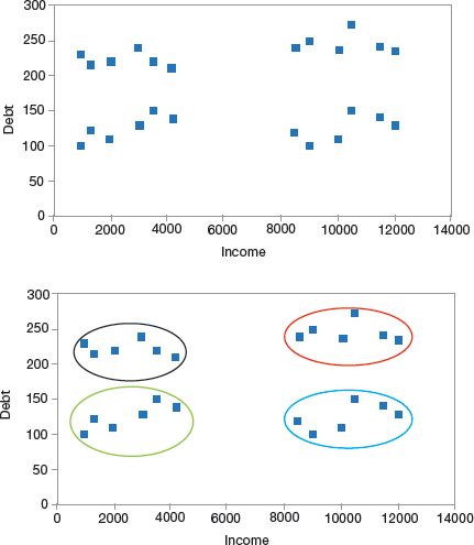
FIGURE 2.20 Cluster of Customers

Income is plotted on the X-axis and the amount of debt is plotted on the Y-axis. A very simple approach is to make four clusters as shown in Fig. 2.20. Looking at Fig. 2.20, we can conclude the following properties of a cluster.

All the data points in a cluster should be similar to each other. In the bank example, such a cluster allows the bank to perform targeted marketing. The data points from different clusters should be as different as possible.

2.5.3 Applications of Clustering in Real-World Scenarios

Clustering is a widely used technique across industry in almost every domain, ranging from banking to recommendation engines, document clustering to image segmentation.

Customer Segmentation

It is to target a specific set of customers or audience in the industry (telecom, e-commerce, sports, advertising, sales, etc.).

Document Clustering

Another very common application of clustering is document clustering in which multiple similar documents are clustered in a similar way as shown in Fig. 2.21.

FIGURE 2.21 Document clustering

Image Segmentation

In image segmentation, similar pixels in the image are clubbed together in the same group (refer Fig. 2.22).

FIGURE 2.22 Image Segmentation

Recommendation Engines

Clustering when used in recommendation engines can help us to recommend songs / friends/ products to our friends.

The algorithm makes a list of things liked by a person and then finds similar things to recommend them to that person.

2.5.4 Evaluation Metrics for Clustering

The goal of any clustering algorithm is not just to make clusters, but to make good and meaningful ones. For example, consider the two cases given in Fig. 2.23.

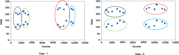
FIGURE 2.23 Different ways of clustering

Since here we have just two features, but in real-world applications, where we have too many features, visualizing all the features together and deciding which clusters are meaningful is just not possible. Therefore, in such a situation, we use evaluation metrics to evaluate the quality of the clusters.

Inertia

Inertia indicates how far the points within a cluster are. For this, sum of distances of all the points within a cluster from the centroid of that cluster is calculated. Once inertia is calculated for all the clusters, the final value of inertia is obtained by adding all these values. This final value that gives the distance within the clusters is known as intra-cluster distance. So, inertia gives us the sum of intra-cluster distances. For best results (or clusters), the inertial value should be as low as possible.

Dunn Index

If the distance between the centroid of a cluster and the points in that cluster is small, it means that the points are closer to each other. So, the inertial value ensures that the first property of clusters is satisfied. However, it does not say anything about the second property – that different clusters should be as different from each other as possible. So, for this, we use the Dunn index.

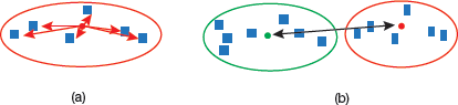
FIGURE 2.24 (a) Intra cluster distance; (b) Inter cluster distance

Along with the distance between the centroid and points, the Dunn index also considers the distance between two clusters. The distance between the centroids of two different clusters is known as inter-cluster distance. The expression for Dunn Index can be given as,

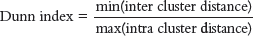
That is, Dunn index is the ratio of the minimum inter-cluster distances and maximum of intra-cluster distances. Its value must be high for getting better clusters.

We must maximize the value of Dunn index. More the value of the Dunn index, better will be the clusters. For a higher Dunn index value, the numerator should be maximum. So, the distance between even the closest clusters should be more so that every cluster is far away from each other. Correspondingly, denominator should be minimum. So, intra-cluster distances should be more.

2.5.5 How K-Means Algorithm Works?

When implementing the k-means clustering algorithm, the following steps are performed.

First specify the number of clusters (k) that will be generated in the final solution. The algorithm starts by randomly selecting k observations (also known as centroids) to serve as the initial centres for the clusters.

In the next step, every remaining observation is assigned to its closest cluster, where closest is a term calculated using the Euclidean distance between the centroid of the cluster and the observation. This step is called ‘cluster assignment step’.

The algorithm then computes the new mean value of each cluster. Therefore, this step is known as ‘centroid update’.

Once the centers are re-calculated, every observation is rechecked to determine its closeness with the same and other clusters. All the observations may have to be reassigned a cluster based on the updated cluster means.

The cluster assignment and centroid update steps are repeatedly performed until the cluster assignments remains the same over iterations (technically, until convergence is achieved).

2.5.6 Pros and Cons of K-Means Algorithm

Pros

1. K-means clustering algorithm is very simple and fast.
2. The algorithm can efficiently deal with very large data sets.

Cons

1. Number of clusters must be pre-specified.
2. The algorithm is sensitive to outliers
3. Changing the order of data will give different results.
4. Create a random data set and then apply the k-means clustering algorithm.

2.5.7 Density-Based Spatial Clustering of Applications with Noise (Dbscan)

We have seen that clustering is an unsupervised learning technique that forms groups of the data points. All points in the same group have similar properties and those in different groups exhibit a different set of properties.

Clusters or groups in data are formed using a variety of distance measures like K-Means (distance between points), affinity propagation (graph distance), mean-shift (distance between points), DBSCAN (distance between nearest points), Gaussian mixtures (Mahalanobis distance to centres), spectral clustering (graph distance), etc.

Though all clustering analysis techniques use the same approach (calculating similarities and then clustering data points into groups), here in this section, we will explore Density-based spatial clustering of applications with noise (DBSCAN) technique.

Why DBSCAN? K-Means clustering, clusters loosely related observations together. Every observation or data point is eventually a part of some cluster even if the observations are scattered far away in the vector space.

The cluster to which an observation will be associated with depends on the mean value of cluster elements. Even a small change in data points may alter the clusters formed. However, this problem is greatly reduced in DBSCAN.

Another issue with k-means algorithm is that you need to specify the number of clusters (‘k’) to be formed and we often err to specify the most optimal value for k. In DBSCAN, the value of k need not be specified. We just need to have an idea about the distance between values and some guidance for what amount of distance is considered ‘close’. DBSCAN produce better results than k-means. This is evident from Fig. 2.25.

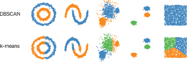
FIGURE 2.25 DBSCAN and k-means Clustering Algorithms

2.5.7.1 Understanding Density-Based Clustering Algorithms

DBSCAN is an unsupervised learning technique that identifies distinct clusters in the data. A cluster is identified as a contiguous region of high point density, separated from other such clusters by contiguous regions of low point density.

The algorithm discovers clusters of different shapes and sizes from a large amount of data that may contain several outlier values.

Two important parameters of the DBSCAN algorithm are discussed here:

minPts which indicates the minimum number of points (a threshold) clustered together for a region to be considered dense.

As a rule of thumb, value of minPts can be derived from the number of dimensions D in the data set. Generally, minPts ≥ D + 1. Setting minPts = 1 is of no use as then every point will form a cluster of its own. With minPts ≤ 2, the result will be similar to hierarchical clustering. Therefore, minimum value of minPts should be at least 3. However, for noisy data sets we must set it to a larger value to get more significant clusters. To be more specific, we can choose minPts = 2·dim to choose larger values for dataset that is very large, or is noisy or contains duplicate values.

eps (ε) is the distance measure that will be used to locate the points in the neighbourhood of any point.

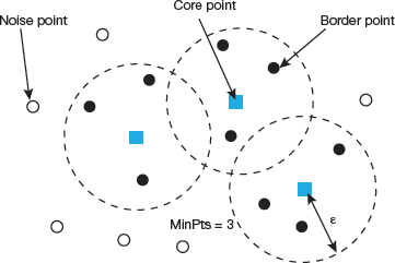
FIGURE 2.26 Terminology used in DBSCAN

The value for ε can be chosen by using a k-distance graph, in which the distance is plotted to the k nearest neighbour ordered from the largest to the smallest value. Here, the value of k can be set to minPts-1. Optimal values of ε can be noted from this plot from the location where an ‘elbow’ is present. If ε is too small, a large part of the data will not be clustered; whereas for a large value of ε, clusters will merge and most of the points will be in the same cluster. However, small values of ε should be preferred to have only a small fraction of points within this distance of each other.

These parameters can be understood by exploring the concepts of density reachability and density connectivity.

Density reachability establishes a point to be reachable from another if it lies within a particular distance (eps) from it.

Connectivity is a transitivity-based chaining-approach that is used to determine points that are located in a particular cluster. For example, a and e points could be connected if a->b->c->d->e, where a->b means b is in the neighbourhood of a.

Once DBSCAN clustering is done, we can recognize three types of points.

Core, it is a point having at least m points within distance n from itself.

Border, is a point having at least one Core point at a distance n.

Noise, is a point that does not fall in the above two categories. This means that noise has less than m points within distance n from itself (refer Fig. 2.26).

2.5.7.2 Algorithmic Steps for Dbscan Clustering

Repeat until all points have been visited.

1. Arbitrarily pick up a point in the dataset ().
2. If there are at least ‘minPoint’ points within a radius of ‘ε’ to the point then all these points are considered to be a part of the same cluster.
3. Expand the clusters by recursively computing the neighbourhood for each point