Decision Trees

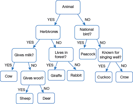
Do you remember the ‘Guess What’ game that we used to play in our childhood? One of us will think of something, and the others had to guess what it is. For that they can ask questions, answers of which will be either ‘Yes’ or ‘No’ based on these clues, the answer is given. For example, consider the tree given in Fig. 2.17. (Note, it is just a sample tree, not a general tree). According to the rules specified, if you are thinking of an animal that is herbivorous and does not live-in forest then it is a rabbit.

FIGURE 2.17 Decision Tree

The same concept is used to create a decision tree for any data science problem. Now, let us study in detail the math behind it.

2.4.2.1 Basic Introduction

Decision tree is one of the most intuitive and popular techniques in data mining that provides explicit rules for classification. It works well with heterogeneous data and predicts the target value of an item by mapping observations about the item.

A decision tree represents choices and their results in form of a tree. The nodes represent an event or choice and the edges of the graph represent the decision rules or conditions. Some common applications of decision tree include the following:

1. Predicting an email as spam or not spam
2. Predicting of a tumour is cancerous or not
3. Predicting a loan as a good or bad
4. Predicting credit risk based on certain factors

Basically, decision trees can perform either classification or regression. For example, identifying a credit card transaction as genuine or fraudulent is an example of classification but using a decision tree to forecast prices of stock would be regression task.

 

Unlike linear models, decision trees map non-linear relationships quite well.

2.4.2.2 Principle of Decision Trees

Decision trees can be used to divide a set of items into n predetermined classes based on a specified criterion. They belong to a class of recursive partitioning algorithms that are simple to describe and implement. To create a decision tree, the following steps are necessary.

Step 1: Select a variable which best separate the classes. Set this variable as the root node.

Step 2: Divide each individual variable into the given classes thereby generating new nodes. Note that decision trees are based on forwarding selection mechanism; so, after a split is created, it cannot be re-visited.

Step 3: Again, select a variable which best separates the classes.

Step 4: Repeat steps 2 and 3 for each node generated until further separation of individuals is not possible.

Now, each terminal (or leaf) node consists of individuals of a single class. That is, once the tree is constructed and division criterion is specified, each individual can be assigned to exactly one leaf. This is determined by the values of the independent variables for the individual.

Moreover, a leaf is assigned to a class if the cost of assigning that leaf to any other class is higher than assigning the leaf to the current class. After all the leaf nodes are assigned a class, we calculate the error rate of the tree (also known as the total cost of tree or risk of the tree) by starting with an error rate of each leaf.

Thus, we see that a decision tree is a supervised learning predictive model that uses rules to calculate a target value. This target value can be either:

• a continuous variable, for regression trees. Such trees are also known as continuous variable decision trees. For example, predict the price of a product or income of a customer (based on his occupation, experience, etc.).
• a categorical variable, for classification trees. Such trees are also known as categorical variable decision tree. Example, to if the target value is ‘Yes’ or ‘No’- whether a customer will buy a product or not.

Programming Tip: Decision tree works for both categorical and continuous input and output variables.

Pruning the Tree

When the decision tree becomes very deep, it must be pruned as it may contain some irrelevant nodes in the leaves. Therefore, pruning avoids creating very small nodes with no real statistical significance.

An algorithm based on decision tree is said to be good if it creates the largest tree and automatically prunes it after detecting the optimal pruning threshold.

The algorithm should also use Cross-validation technique and combine error rates found for all possible sub-trees to choose the best sub-tree.

 

A tree with each node having no more than two child nodes is called binary tree.

For example, if information gain of a node is −10 (loss of 10) and then the next split on that gives us IG of 20, then a simple decision tree will stop at step 1 but in pruning, the overall gain would be taken as +10 and both the leaves will be retained.

2.4.2.3 Key Terminology

Some important terms that are frequently used in decision trees (and demonstrated in Fig. 2.18) are as follows:

1. Root node: This is the node that performs the first split.
2. Terminal nodes/Leaves: These nodes predict the outcome.
3. Branches: They are depicted by arrows that connect nodes and shows the flow from question to answer. Technically, a branch is a sub section of entire tree
4. Splitting: This is the process of dividing a node into two or more sub-nodes. In a decision tree, splitting done until a user-defined stopping-criteria is reached. For example, the programmer may specify that the algorithm should stop once the number of items per node becomes less than 30. 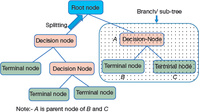FIGURE 2.18
5. Decision node: This is a sub-node that splits into further sub-nodes
6. Terminal or Leaf node: It is a sub-node that does not split further.
7. Parent node: A node which splits into sub-nodes is called a parent node of the sub-nodes (or child of the parent node).

2.4.2.4 Advantages of Decision Trees

Decision trees are one of the most popular statistical techniques because it provides following advantages to users.

1. It is easy to implement
2. Results can be easily understood. It does not require any statistical knowledge to read and interpret them.
3. Programmers can code the resulting model
4. It executes faster when the model is applied to new individuals.
5. Outliers or extreme individuals can not affect decision trees.
6. Some decision tree algorithms can deal with missing data.
7. A decision tree allows users to visualize the results and represents all factors that are important in decision making.
8. Decision trees provide a clear picture of the underlying structure in data and relationships between variables.
9. They can also be used to identify the most significant variables in the data-set
10. Decision trees closely mirror human decision-making compared to other regression and classification approaches.
11. Decision trees requires less data cleaning as compared to other techniques.
12. They are not influenced by missing values to a fair degree.
13. They can handle both numerical as well as categorical variables.
14. Decision trees employs non parametric method as they have no assumptions about the space distribution and the classifier structure.

 

OUTLIERS

An outlier is an individual data item or observation that lies at an abnormal distance from other data values in a random sample of a data set. It is the work of the data analyst to decide what will be considered abnormal. Outliers should be carefully investigated as they may contain valuable information about the data being processed. Data analyst must be able to answer questions like the reasons for the presence of outliers in the data set, probability that such values will continue to appear, etc. for example, if an examination was held of maximum marks 100, then one or more students getting more than 100 will be treated as an outlier.

Outlier analysis is extensively used for detecting fraudulent cases. In some cases, outliers may be contextual outliers. This means that a particular data value is an outlier only under a specific condition. For example, in hot summer season when temperature is 40 degrees and above, then an unexpected windstorm and rain may bring it to 32 degrees. Another example could be that a bank customer may not be withdrawing more than 50K in a month but because of a family wedding may withdraw 2.5 lakhs in a day.

2.4.2.5 Limitations of Decision Trees

The disadvantages of using decision trees are as follows:

1. The tree detects local, not global, optima.
2. All independent variables are evaluated sequentially, not simultaneously.
3. The modification of a single variable may change the whole tree if this variable is located near the top of the tree.
4. Decision trees lack robustness. Though this can be overcome by resampling, in which one can construct the trees on many successive samples and can aggregate by mean, but this will lead to a complex tree that is difficult to read and interpret. The problem of overfitting can be done by tree pruning and setting constraints on tree size.
5. Since each split reduces the number of remaining records, later splits are based on very few records have less statistical power.
6. The property of forwarding variable selection and constant splits of nodes makes prediction by trees not as accurate as done by other algorithms.
7. Overfitting is a key challenge in modelling decision trees. If there is no limit set of a decision tree, it will give 100% accuracy on training set because in the worst case, there will be a single leaf for each observation.