
Data science has progressed from simple linear regression models to complex techniques but practitioners still prefer the models that are simple and easy to interpret. In this widely used category of algorithms Naïve Bayes algorithm is one of the prominent names as it is not only simple but so powerful that it outperforms complex algorithms for very large datasets.
Naive Bayes is a probabilistic machine learning algorithm based on the Bayes Theorem. This algorithm is extensively used in a wide range of classification tasks varying from filtering spam, classifying documents to predicting sentiments.
Programming Tip: The tern naïve means that features that are used in the model are independent of each other. So when one feature change, the other is not affected.
2.6.1 Understanding Conditional Probability
To understand conditional probability, consider an example of flipping a coin. There are equal chances of getting either heads or tails. So, the probability of getting heads is 50%.
Now, in case we are supposed to find the probability of getting a queen spade from a deck of 52 cards then the denominator is 13 (the eligible population) and not 52. Since there is only one queen in 13 spades, the probability that we get a queen spade is 1/13.
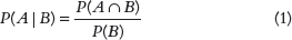
Therefore, we can say that the conditional probability of A given B, denotes the probability of occurring A given that B has already occurred. Mathematically, it can be expressed as, P(A|B) = P(A AND B) / P(B).
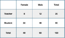
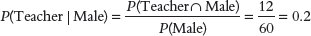
Let’s apply this concept on the data set given in Fig. 2.27 and calculate the conditional probability that the teacher is a male.
So, the required conditional probability P(Teacher | Male) = 12 / 60 = 0.2.
Programming Tip: If Y has two categories, then calculate the probability of each class of Y and select the one with higher value.
Likewise, the conditional probability of B given A can be computed as,

2.6.2 The Bayes Rule
The Bayes Rule uses P(X|Y), known from the training dataset, to find P(Y|X). For observations in test dataset, X would be known while Y is unknown. And for each row of the test dataset, we have to find the probability of Y given that X has already happened (refer Fig. 2.28).
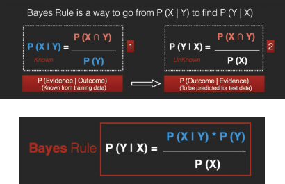
FIGURE 2.28 Bayes Rule for Conditional Probability
2.6.3 Types of Events
If two probabilities, P(B) and P(B|A) are the same, then it means that the occurrence of event A had no effect on event B. Therefore, event A and event B are independent events.
If the conditional probability is zero, then it means that the occurrence of event A implies that event B cannot occur. If the reverse is also true, then the events are said to be mutually exclusive events. In such a case, only one event can take place at a time.
All other cases are classified as dependent events where the conditional probability can be either lower or higher than the original.
For example, if we toss a coin twice and we want to calculate the probability of getting a head both times, then we must consider that the second event is independent of the first. The desired probability is P(Heads in first throw)![]() P(Heads in second throw)= ½ X ½ = ¼
P(Heads in second throw)= ½ X ½ = ¼
Mathematically, we can say that if the events are not independent, we multiply the probability of one event with the probability of the second event.
For expressing dependent events mathematically, we multiply the probability of any one event with the probability of the second event after the first has happened.
P(A and B)=P(A)![]() P(B|A) or P(A and B)=P(B)
P(B|A) or P(A and B)=P(B)![]() P(A|B)
P(A|B)
For example, while drawing two cards (King and Queen) without replacement, the probability of the first event is dependent of 52 cards whereas the probability of the second event is dependent on 51 cards.
This means that P(King and Queen)=P(Queen)P(King|Queen)
So if P(Queen) is 4/52 then once the King is drawn, P(King|Queen) is 4/51 as now only 51 cards are left. Therefore, the desired probability = 4/52 X 4/51
The probability of two non-mutually exclusive events is given as, P(A OR B)=P(A) + P(B) – P(A AND B).
For example, in a throw of dice, the probability of getting a number that is multiple of 2 or 3 is a scenario of events which are not mutually exclusive since 6 is both a multiple of 2 and 3 and is counted twice. Therefore, P(multiple of 2 or 3) = P(Multiple of 2) + P(Multiple of 3) – P(Multiple of 2 AND 3) = P(2, 4, 6) + P(3, 6) – P(6) = 3/6 + 2/6 -1/6 = 4/6 = 2/3
2.6.4 Naive Bayes Algorithm
In real-world problems, there are multiple X variables. So, when the features are independent, the Bayes Rule can be extended to what is called Naive Bayes. It is called ‘Naive’ because of the naive assumption that the Xs are independent of each other.
Naive Bayes classification algorithm can be used with continuous features but performs best for categorical variables. When dealing with numeric features, the algorithm assumes that numerical values are normally distributed.
2.6.5 Laplace Correction
We can better understand the importance of Laplace correction with an example. If we were to classify fruits as mango, orange or banana, then the value of P(Long | Orange) will be zero as there are no ‘Long’ oranges.
When we use this probability in the model having multiple features, then the entire probability will become zero as anything multiplied by zero is zero. To avoid this, we need to increase the count of the variable with zero to a small value (usually 1) in the numerator, so that the overall probability does not become zero.
This correction is called ‘Laplace Correction and the function for building the Naive Bayes model will accept this correction as a parameter.
2.6.6 Pros and Cons of Naive Bayes Algorithm
Pros
- It is a simple algorithm that is easy to build and understand.
- It predicts classes faster than many other classification algorithms.
- It can be easily trained using a small data set.
- It can be used to predict values for even large data sets.
Cons
- If a given class and a feature has 0 frequency, then the conditional probability will become 0 resulting in the ‘Zero Conditional Probability Problem.’ This is a serious issue as it wipes out all other vital information about probabilities. However, to avoid such situations there are several sample correction techniques like the ‘Laplacian Correction.’
- Another disadvantage is the very strong assumption of independence class features that it makes. It is near to impossible to find such data sets in real life.
2.6.7 Applications
Some of the real-world scenarios where Naive Bayes algorithm is used include the following:
- Text classification: Naïve Bayes classification algorithm is one of the most preferred algorithms to classify whether a text document belongs to one or more categories (classes).
- Spam filtration: Many popular email services uses the Bayesian spam filtering to distinguish spam email from legitimate email. Many server-side email filters like DSPAM, SpamBayes, SpamAssassin, Bogofilter, and ASSP are all based on Naïve Bayes classification technique.
- Sentiment Analysis: The Naïve Bayes algorithm is also used to analyse the analyse tweets, comments, and reviews posted on social networking site to classify as being negative, positive or neutral.
- Recommendation System: Companies uses recommendation systems to predict whether a particular user will like their product and/ or buy their product or not. For this, the Naive Bayes algorithm is used in conjunction with collaborative filtering techniques to build hybrid recommendation systems.
Leave a Reply