
Regression analysis is a statistical method tool that allow users to study the relationship between a dependent (target) and one or more independent (predictor) variables as shown in Fig. 2.10. This helps the analyst to understand how the value of the dependent variable changes with respect to independent variables. The values to be predicted are usually continuous or real (like temperature, age, salary, price, etc.). For example, a company can analyse its data to find out the extent to which expenditure on advertisements increases sales of a particular product. Similarly, we can use regression analysis to predict rainfall using temperature and other factors; determine market trends; predict road accidents due to rash driving.
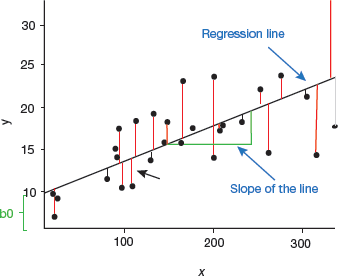
FIGURE 2.10 Plotting the Regression Line
Regression analysis is widely used for prediction, forecasting, modelling time series data, and inferring the causal-effect relationship between variables.
In regression analysis, a graph that best fits the given datapoints is plotted. This graph can either have a straight line or a curve that passes through all the datapoints on the graph that is drawn depicting the dependent and independent variable(s). The vertical distance between the datapoints and the regression line should be minimum as this line indicates whether the model has captured a strong relationship or not.
2.3.1 How Regression Analysis Works?
Regression analysis creates a mathematical equation that defines y as a function of the x variables. This equation is then used to predict the value of y on the basis of values of the predictor variables (x).
Linear regression is the most basic, simple and widely used technique for predicting values of a continuous variable. It assumes that there exists a linear relationship between the outcome and the predictor variables as shown in Fig. 2.11.
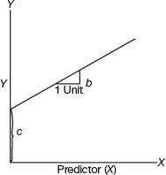
FIGURE 2.11 Relationship between outcome and predictor variable
The linear regression equation can be given as,

b0 is the intercept,
b is the coefficient of x.
e is the residual error
Values of coefficients are determined in such a way that the residual error is minimized. This method of computing the beta coefficients is known as ordinary least squares (OLS) method.
In case of multiple predictor variables, say x1 and x2, the regression equation can be written as y = b0 + b1x1 + b2x2 +e. There may also exist an interaction effect between two or more predictor variables. For example, increasing the value of one predictor variable may in turn increase the effectiveness of the other predictor(s) in explaining the variation in the outcome variable.
When there are multiple predictors in the regression model, then the best combination of predictors needs to be chosen (like best subsets regression and stepwise regression) to construct the optimal predictive model. In such cases, we use model selection technique that compares multiple models built with different sets of predictors to select the best performing model that minimizes the prediction error.
Linear regression models work well with both continuous and categorical predictor variables. However, before applying linear regression model on our data set, we must first make sure that the linear model is suitable for the underlying data. It may happen that the relationship between the outcome and the predictor variables is not linear. In such cases, a non-linear regression model (like polynomial and spline regression) is preferred over a linear model.
When there is a large multivariate data set containing some correlated predictors, then such variables are summarized into few new variables that are a linear combination of the original variables. These techniques based on principal components include principal component regression and partial least squares regression. Alternatively, we can use penalized regression to simplify a large multivariate model. Such a regression model penalizes the model for having too many variables. Ridge regression and Lasso regression are popular examples of penalized regression model.
Thus, different regression models can be applied on the data and their performance can be compared to select the best one that explains the data. Statistical metrics are used to compare the performance of the different models in explaining the data and predicting the outcome of new test data.
Case Study 1: Let us compute auto fare. We know that auto charges are computed by adding a fixed amount and a variable cost. The fixed amount is set by the government. The variable cost depends on the distance travelled. It is usually specified as Rs 11 per km. If the fixed charge of an auto is Rs 30, then a linear regression equation can be used to find the cost of any auto trip. By using “x” to represent the number of kilometers travelled, “y”, the cost of that auto ride can be calculated as, y = 11x + 30.
Now, if I say that I took an auto to reach a destination that was 10 km away from my house, how much would I have to pay? Yes, Rs. 140. Because, y (cost) = 11 X 10 + 30.
Case Study 2: A company decides to carry out its business operations on a rented space. If the cost of the rental space is Rs 20000 plus Rs 500 per employee per day, then compute monthly rental for space given that the company is open 5 days a week.
The linear equation in this scenario, can be given as,
y = (500)(5)(4)x + 20000
y = 10000x + 20000
If 20 employees are to be present every day, then monthly rental would be
Y (cost) = 10000 X 20 + 20000 = 220000.
Case Study 3: Let us make predictions using simple linear regression equation. If the annual expenditure of a bakery shop is Rs 500000 and the monthly sales is Rs 450000, then the linear equation to compute profit for x months can be given as,
y = 450000x − 500000
For example, after six months, the shop can expect a profit of,
450000![]() 6 − 500000 = 2200000.
6 − 500000 = 2200000.
2.3.2 Model Evaluation Metrics
The best regression model is the one with the lowest prediction error. The most widely used metrics for comparing regression models are discussed here:
Root mean squared error measures the model prediction error. It is calculated as the average difference between the observed known values of the outcome and the predicted value by the model. Mathematically,

Lower the RMSE, better is the model.
Adjusted R-square represents the proportion of variation in the data thereby reflecting the overall quality of the model. Higher the adjusted R2, better is the model
These metrics are computed on a new test data that has not been used to train or build the model. In a large data set with many records, rows can be randomly split in 80:20 ratio, where 80% of the rows are used to build the predictive model and rest of the 20% are used as test set or validation set for evaluating the model performance.
One of the best techniques for estimating a model’s performance is k-fold cross-validation. This can be applied even on a small data set. Step followed to perform k-fold cross-validation are as follows:
Step 1: Randomly split the data set into k-subsets (or k-fold). For example, to generate 5 subsets, value of k = 5.
Step 2: Reserve one subset and call it as test data. Use rest of subsets to the train the model.
Step 3: Test the performance of the model using the test data set and record the prediction error
Step 4: Repeat the above steps until each of the k subsets have been used as the test set.
Step 5: Calculate the average of the k recorded errors. This is also known as cross-validation error. Finally, the best model is the one that has the lowest cross-validation error, RMSE.
2.3.3 Types of Regression
The type of regression analysis that can be applied on a particular data set depends on the attributes, target variables, shape and nature of the regression curve that represent the relationship between dependent and independent variables. Some important regression techniques are as follows:
- Linear regression: It is the simplest regression technique used for predicting values for a dependent variable that has linear relationship between the response and predictors (or descriptive variables). The general equation of linear regression can be given as,
 where Y is a dependent variableX is the independent variableb is the slope of the regression line andC is the intercept.Though linear regression suffers from overfitting issues, it is still used as it is fast and easy to model and evaluate. It is best used when the target relationship is not complex or enough data is not available. Linear regression (Fig. 2.12) is also very useful for detecting outliers.
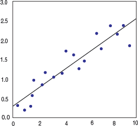 FIGURE 2.12 Linear Regression Graph
 - Logistic regression: It is preferred when the dependent variable is binary (dichotomous) in nature (like 0 or 1, true or false, yes or no). That is, logistic regression is preferred when there is a need to ascertain the probability of an event in terms of either success or failure. In such a case, the relationship between the dependent and independent variables are calculated by computing probabilities using the logit function (refer Fig. 2.13). Logistic regression is mostly used to analyse categorical data.
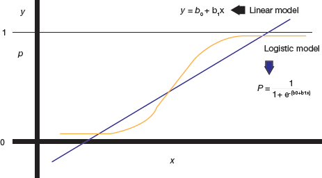 FIGURE 2.13 Logistic Regression Curve
 - Ridge regression: Ridge regression is basically used for analysing numerous regression data. In case of multicollinearity, least-square calculations get unbiased, so the regression model becomes too complex and approaches to overfit. In such a case, we need to minimize the variance in the model and save it from overfitting. Ridge regression helps us to do this by correcting the size of the coefficients. A bias degree is affixed to the regression calculations that in turn reduces standard errors.
- Lasso (Least Absolute Shrinkage Selector Operator) regression: It is a widely used regression analysis technique for variable selection and regularization. Lasso regression uses thresholds to select a subset of the covariates given for the implementation of the final model. It reduces the number of dependent variables if the penalty term is huge. This is done by reducing the coefficients to zero so that features can be selected easily. Lasso regression is also known as L1 regularization. Ridge regression eases collinearity in between predictors of a model
- Polynomial regression: Polynomial regression is used to construct a model that fits non-linearly separated data. In such a case, the best-fitted line is not a straight line, but a curve.The equation of polynomial regression is given as, Y=b0+b1x1+b2x22+……..bn xnnPolynomial regression is widely used to analyse curvilinear form of data (refer Fig. 2.14) and best fitted for least-squares methods.
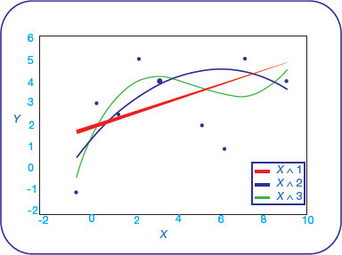 FIGURE 2.14 Polynomial Regression Curve
 - Stepwise regression: It is used to build predictive regression models that are carried out naturally. With every forward step, a variable gets added or subtracted from a group of descriptive variables.We can use forward selection, backward elimination or bidirectional elimination for adding/removing variables at each step. As the name suggests, forward selection continuously adds variables to the set and reviews the performance of the model. It stops when no further improvement is needed (or being achieved). Backward elimination removes variables until no extra variable is left to be deleted without considerable loss. Bidirectional elimination is a good combination of both the approaches.
- ElasticNet regression: Elastic regression is a mix of ridge and lasso regression. It produces a grouping effect when highly correlated predictors are either in or out in the model combinedly. This technique is preferred when there are too many predictors as compared to the number of observations. ElasticNet regression is usually used in SVM (Support Vector Machine Algorithm), metric training, and document optimizations.
Leave a Reply