
For a long time historically, computation was a matter of actually solving,
or finding algorithms to solve, various mathematical problems using mechan-
ical or other algorithms. It was only in the early twentieth century that the
process of computation was modelled in mathematical terms, largely in the
works of Alan Turing, Alonso Church, Kurt G¨odel, and Emil Post. Their efforts
were directed at extracting the basic properties of a computational process,
independent of the platform on which it was executed.
The first question regarding computation that a theoretician asks is
whether or not the given problem is computable. What exactly does this mean?
If the problem is somehow reduced to the calculation of a function, then is this
function computable? In order to meaningfully answer this question without
having to examine all possible algorithms designed to compute the function,
the famous mathematician Alan Turing came up with a theoretical model
computer known as the Turing Machine, which is a simplification of your
desktop computer to the bare bones.
101
102 Introduction to Quantum Physics and Information Processing
6.1.1 Turing machine
Turing’s abstract computing machine captures the concept of an algorithm
to evaluate a function. It can be thought of as a mechanical analogue of an
algorithm broken down to its bare bones. Now an algorithm basically takes
an input in some symbolic form, performs basic manipulations in steps that
may even be recursive and finally finishes up with an output. In the paradigm
of a computing machine, the machine has a means of accepting and reading
an input, a set of instructions on what basic steps to perform, which may
depend on the output at a previous step. The machine must therefore be able
to move back and forth over previous steps and write out the answer at
each step, and halt when the process is over. This mechanism of comparing
outputs to conditions in the program can be achieved easily by attributing an
internal state to the machine.
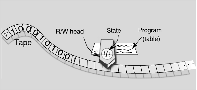
FIGURE 6.1: A schematic of a Turing machine.
Turing modelled this process in an abstract machine (TM), schematically
shown in Figure 6.1, consisting of the following.
1. A tape which is a string of cells that can contain one of a finite set of
symbols, Γ = {S
i
}, which could, for example, be binary 0 and 1, a blank
(
0) and a special symbol B, for the left edge of the tape.
2. A read/write head that can take input from or write output to a cell
at a time when fed into the machine.
3. A register that stores the internal state of the machine, which could
be one of a finite set of states {q
i
}. There are two special states, S, the
starting state and H, the halting state.
4. A table of instructions (like a program) that make the head execute
a Left move, a Right move, and a Print, depending on the symbol
currently read by the head. This is like a function f(q, x) = hq
0
, x
0
, mi
Computation Models and Computational Complexity 103
where q is the current state of the machine, x is the current symbol read,
q
0
is the new state after execution of the step, x
0
is the symbol written
on to the tape, and m is a move L, R, or 0.
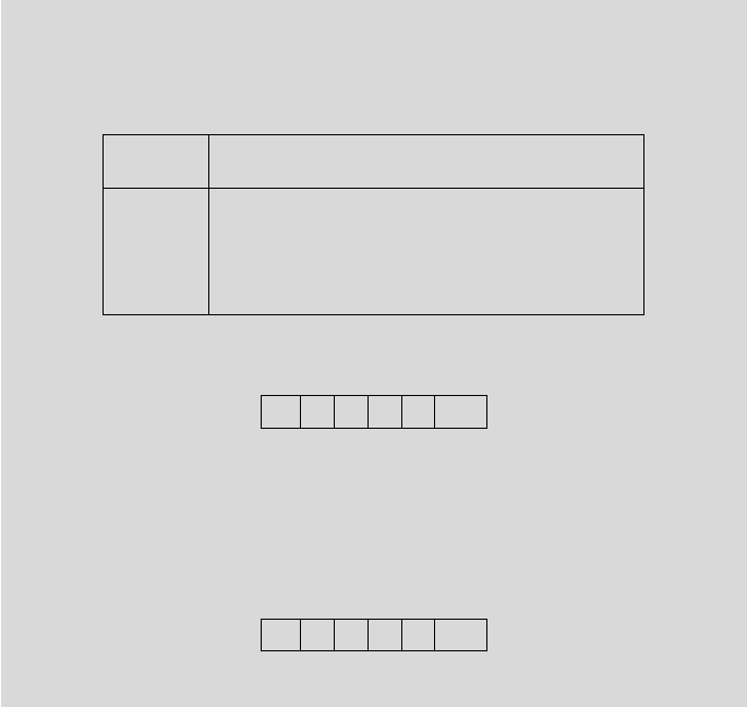
Example 6.1.1. To see how a TM might work, consider one with binary
symbols, Γ = {0, 1,
0, B} and internal states Q = {S, q
1
, q
2
, q
3
, H}. Let the
table (program) be as follows:
H
H
H
H
H
x
q
i
B 0 1
0
S hq
1
, B, Ri
q
1
hq
1
, 0, Ri hq
1
, 1, Ri, hq
2
,
0, Li
q
2
hq
3
,
0, Li, hq
3
,
0, Li
q
3
hH, B, 0i hq
3
, 0, Li, hq
3
, 1, Li hH,
0, Li
Can you see what this machine achieves? Take for example an input string
110 on the tape followed by blanks. The tape would look like
B 1 1 0
0 . . .
The sequence of states followed by the machine are:
hS, Bi → hq
1
, Bi
R
−→ hq
1
, 1i
R
−→ hq
1
, 1i
R
−→ hq
1
, 0i
R
−→ hq
2
,
0i
R
−→ hq
3
,
0i
L
−→ hq
3
, 1i
L
−→ hq
3
Bi → hH, Bi.
The tape now looks like
B 1 1
0
0 . . .
You can see that this machine erases the last symbol on the tape. Try it
out on a different input.
Exercise 6.1. Try to construct the table of instructions for a TM that adds 1 to
the entry on the tape.
Every TM is specified by its own set of symbols Γ, set of internal states
Q, and program. So there exists a specific Turing machine for every specific
algorithm. However, the machine may be made programmable according to
different algorithms, if the program is also fed in as part of the input. Thus a
programmable Turing machine can simulate any other Turing machine: this
is the universal Turing machine (UTM).
In his work, strengthened by the work of Alonso Church, who was simulta-
neously working on Hilbert’s famous computability problem, Turing was able
to prove the thesis that any algorithm could be simulated by a UTM. Church’s
work strengthened this to the Church–Turing thesis:
104 Introduction to Quantum Physics and Information Processing
Theorem 6.1. Any function that can be computed by an algorithm can be
efficiently simulated by the Universal Turing Machine.
Turing was then able to formulate the problem of computability in terms
of whether or not such a universal machine would halt, i.e., find a solution. So
problems on which this machine halted would then be called computable.
Interestingly enough, the famous halting problem, viz. whether or not a
particular algorithm on a Turing machine will halt, is itself uncomputable!
The question then begged to be asked as to whether a given problem that
is not computable by a UTM can be made so by a different paradigm of com-
putation. This led to extensions of the Turing machine concept to probabilistic
Turing machines where the algorithms made use of fuzzy logic.
6.1.2 Probabilistic Turing Machine
One of the major challenges to the Church–Turing thesis came from al-
gorithms that were probabilistic, that is, could solve problems efficiently but
with a certain (bounded) probability of failure. These problems, for instance
the Solovay–Strassen primality test (1977) cannot be efficiently solved on the
deterministic Turing machine described above.
Computer scientists therefore extended the validity of the Church–Turing
thesis to probabilistic algorithms by designing a probabilistic Universal Turing
Machine.
A probabilistic or randomized Turing machine is one in which randomness
is built into each step which chooses possible options according to a probability
distribution. Such a machine therefore would need to have an additional tape:
the random tape, containing a string of random numbers to decide the options
at each step. Without going into details, we will state that a probabilistic
universal Turing machine (PTM) can replace the earlier deterministic one
to save the Church–Turing Thesis in its stronger form.
There is a plethora of randomized complexity classes that can be defined
for randomized algorithms that we will not go into, but this extends the class
of efficiently solvable problems.
6.1.3 Quantum Turing Machine
The challenge to this model of computation came with trying to simulate
quantum mechanical systems on a PTM; this was still unsolvable. The natural
question to ask was whether or not it was possible to generalize to a quantum
Turing machine (QTM) that would further expand the class of solvable
problems. This was done by David Deutsch in 1985 though thought of earlier
by Benioff and Bennett.
The most important idea behind this machine, which is also probabilistic,
is that it is reversible, in the same way as quantum time evolution is reversible.
The idea behind discussing Turing models is to see if the class of problems
Computation Models and Computational Complexity 105
that are hard to solve can be made smaller. As it turned out, while QTMs
cannot reduce the class of unsolvable problems, they do reduce that of hard
problems.
The Turing model is the most mathematically abstract model for compu-
tation, and is widely used to establish computability and upper bounds on
the efficiency of a given algorithm. There are several other models involving
for example, decision trees, cellular automata, or logical calculus. The most
practical approach is called the circuit model where elementary logic opera-
tions are used as building blocks to evaluate the function. It was shown that
the circuit model was equivalent to the Turing model, so that there is no loss
in generality in concentrating on this, as we will in most of this book
Leave a Reply