A simple extension to this algorithm works when the search criterion has
multiple solutions. The oracle then gives an answer “yes” whenever any one
of the M possible solutions is input. The Hilbert space then has a “solution
subspace” M, spanned by M solution states. Let us denote by |βi the uniform
superposition of all these vectors, and by |αi, its orthogonal complement.
|βi =
1
√
M
X
x∈M
|xi, (8.81)
|αi =
1
√
N − M
X
x /∈M
|xi. (8.82)
In this situation, the input state is
|ψi =
r
M
N
|βi +
r
N − M
N
|αi. (8.83)
The angle θ is now given by
sin θ = hψ|βi =
r
M
N
. (8.84)
The operator
ˆ
O tags all of the M solutions with a ‘−’ sign, and the Grover
iterate is defined the same way as before. After p iterations we get the state
ˆ
G
p
|ψi = cos[(2p + 1)θ]|αi + sin[(2p + 1)θ]|βi, (8.85)
and the number of iterations required is nearly
p ≈
π
4
r
N
M
. (8.86)
You should check for yourself that this works out.
172 Introduction to Quantum Physics and Information Processing
8.6.2 Quantum counting
A fallout of the multiple search algorithm is the counting algorithm. Be-
fore we know how many times to iterate, we need to know how many solutions
M there are to the search criterion. Can we deduce a quantum algorithm for
finding M given U
f
k
? The solution found by Brassard et al. [15], is a com-
bination of Grover’s search and Shor’s phase estimation algorithms. The key
point here is to note that the number of solutions is related to the eigenvalues
of the operator
ˆ
G, which can also be expressed in the |αi-|βi basis as the 2-d
matrix
ˆ
G =
cos ϕ −sin ϕ
sin ϕ cos ϕ
!
where sin ϕ = 2
p
M(N − M)
N
. (8.87)
The eigenvalues of this matrix are e
±iϕ
. We can therefore use the phase estima-
tion algorithm to deduce ϕ. We need to feed the algorithm with an eigenstate
of
ˆ
G. Now you can see for yourself that |ψi is a linear superposition of the two
eigenstates of
ˆ
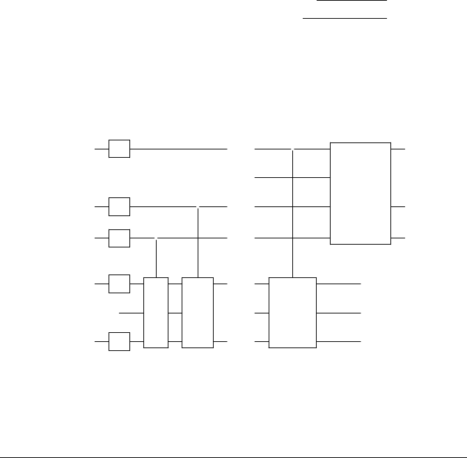
G, so the circuit of Figure 8.18 will work to t bits of accuracy.
|0i
H
. . .
•
QF T
−1
.
.
.
.
.
.
.
.
.
.
.
.
.
.
.
t qubits |0i
H
•
. . .
|0i
H
•
. . .
|0i
H
ˆ
G
G
2
. . .
G
2
t−1
n + 1 qubits
.
.
.
.
.
.
.
.
.
|0i
H
. . .
FIGURE 8.18: Circuit for quantum counting
Leave a Reply