Two qubits together can be represented as 4-column vectors in Hilbert
space. The most general 2-qubit gate is therefore a 4×4 unitary. An operation
on two qubits that acts independently on each of the two can be expressed as
a direct product of two single-qubit operations as defined in Equation 3.31:
O = O
1
⊗ O
2
.
For example, the 2-qubit H gate is represented by the action
H
⊗2
|xi|yi = H|xi ⊗ H|yi, (7.14)
with matrix representation
1
2
“
1 1
1 −1
#
⊗
“
1 1
1 −1
#
=
1
2
1 1 1 1
1 −1 1 −1
1 1 −1 −1
1 −1 −1 1
. (7.15)
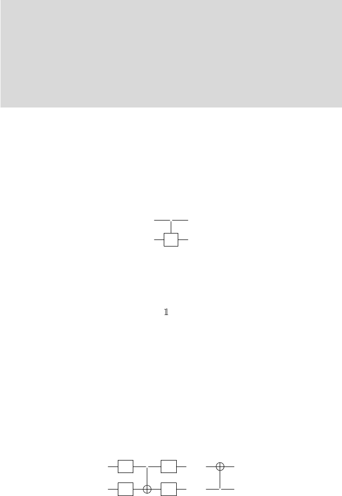
You need to distinguish between the different possibilities shown in Figure
7.4. The circuit diagrams for these gates will clarify the difference.
H ⊗ H ⊗ H ⊗ H
H H
H
H
FIGURE 7.4: H gates acting in different ways on two qubits.
These sort of gates can easily be generalized to any dimensions.
Exercise 7.9. Construct the matrix representations for the operators shown in
Figure 7.4.
Exercise 7.10. Find the matrix representing X ⊗ Z.
128 Introduction to Quantum Physics and Information Processing
The interesting thing about multi-qubit gates is that in general, they would
not act independently on the individual qubits, but entangle them. This is
the hallmark of quantum information processing that gives the most crucial
advantage over classical processing. For example, consider the most famous
2-qubit gate, the controlled-NOT or CNOT gate whose classical version we
saw in Chapter 6. This gate flips the target qubit when the control qubit is set
to 1. The truth table of the CNOT is used to define the action of the quantum
gate on the computational basis states:
U
CNOT
=
1 0 0 0
0 1 0 0
0 0 0 1
0 0 1 0
≡
“
0
0 X
#
(7.16)
Notice that the truth table for the second output corresponds to the well-
known XOR operation on the inputs. The operation is, however, completely
reversible. We denote the action of this gate by
U
CNOT
|xi|yi = |xi|x ⊕ yi. (7.17)
Note that when we use letters x and y to label quantum states, they refer to the
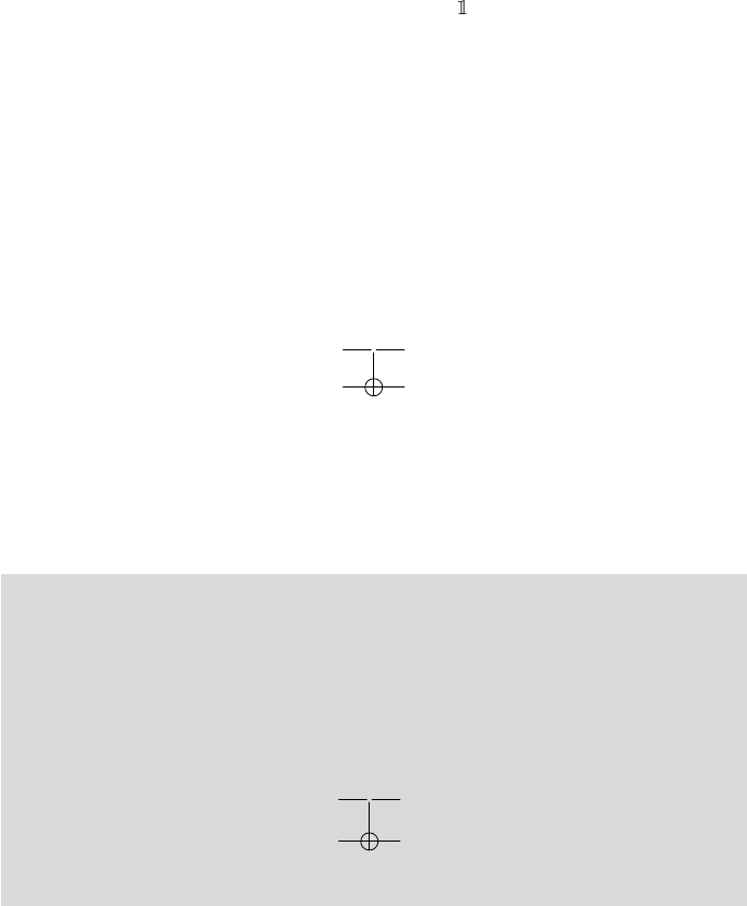
computational basis states. This gate is represented by the circuit of Figure 7.5.
An important caveat here: though the control qubit seems to come out of the
|xi
•
|xi
|yi |x ⊕ yi
FIGURE 7.5: CNOT gate.
gate unchanged when it is in a computational basis state, the output will in
general be entangled with the state of the target qubit, as we will see in the
next example.
Example 7.2.1. As an illustration of how a controlled gate acts on superpo-
sition states, consider
CN OT (α|0i + β|1i)|0i = CNOT (α|00i + β|10i)
= α|00i + β|11i (7.18)
which is an entangled state. Figure 7.6 gives the circuit for this process.
α|0i + β|1i
•
α|00i + β|11i
|0i
FIGURE 7.6: CNOT producing entanglement.
Quantum Gates and Circuits 129
This example also illustrates the No-cloning theorem of Chapter 4. The CNOT
gate appears as a cloner if the target qubit is |0i:
U
CNOT
|xi|0i = |xi|xi. (7.19)
However, this is true iff |xi is a computational basis state. If the control qubit
is a generic quantum state |ψi, the output of this gate is an entangled state.
If our gate were a cloner, then the output ought to have been |ψi⊗|ψi, which
is a separable state.
The notion of a conditional or controlled gate can be extended to any
unitary single-qubit operation U by defining
U
CU
|xi|yi = |xiU
x
|yi (7.20)
The notation makes it obvious that the operator U acts on the target qubit |yi
only if the control qubit is set to 1. Figure 7.7 shows the circuit representation
for this action.
|xi
•
|xi
|yi
U
U
x
|yi
FIGURE 7.7: Circuit representing a controlled-U gate.
The matrix representation of such a gate is
U
CU
=
“
0
0 U
#
. (7.21)
You can prove that U
CU
is unitary if U is.
One can use either of the input qubits as the control or the target. We will
use the notation C
ij
to denote the i
th
bit as the control bit and the j
th
bit as
the target.
Exercise 7.11. Show that (H ⊗H)C
12
(H ⊗H) = C
21
, i.e., if you change basis
from computational basis to the X basis {|+i, |−i}, then the control and
target bits get interchanged. The circuit for the problem looks like Figure
7.8.
H
•
H
≡
H H
•
FIGURE 7.8: CNOT with second qubit as control and first as target.
130 Introduction to Quantum Physics and Information Processing
X
•
X
≡
FIGURE 7.9: A 0-controlled gate.
The control action can be conditioned on the control bit set to 0 instead
of 1. Such a gate is represented in Figure 7.9.
For more than one qubit, a variety of control possibilities are illustrated
in Figure 7.10.
Multiple target CNOT
• • •
≡
Multiple control (CCNOT):
•
•
(No simple equivalent)
FIGURE 7.10: Different control operations
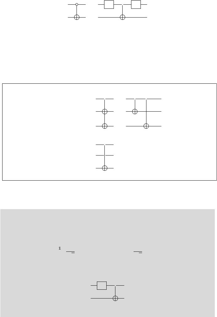
Example 7.2.2. Creating Bell states
Prototype entangled states are the Bell states of Equation 4.10, and they
can be produced using CNOT gates. For example,
|0i ⊗ |0i
H⊗
−−−→
1
√
2
(|0i + |1i) ⊗ |0i
C
12
−−→
1
√
2
(|00i + |11i), (7.22)
producing the first Bell state |β
00
i. It’s easy to deduce that the general Bell
state is produced by the simple circuit given in Figure 7.11:
|xi
H
•
|β
xy
i
|yi
FIGURE 7.11: Circuit for preparing Bell States
Exercise 7.12. Verify that the operation depicted in circuit 7.11 is reversible
Leave a Reply