
Applications
The Fourier transform, a mathematical tool named after the 18th century
French mathematician Joseph Fourier, is an invaluable tool in engineering
and the sciences. No technical education is complete without a firm grasp
of this technique and its uses. The simplest way to understand the Fourier
transform F of a function f (x) is to imagine the function as made up of
various components that are periodic (like a sine function) with a frequency
y, and F(f(x)) as a function
˜
f(y) measuring the amplitude of each frequency
component in the function. In other words, we construct a decomposition
of the function in terms of the oscillatory exponential e
−2πiyx
, where the
coefficients in that decomposition are the Fourier transform:
f(x) =
1
√
2π
Z
∞
−∞
dy e
2πiyx
˜
f(y). (8.19)
This formula is said to define the inverse Fourier transform of
˜
f(y), while the
Fourier transform is defined as
F(f(x)) =
˜
f(y) =
1
√
2π
Z
∞
−∞
dx e
−2πiyx
f(x). (8.20)
The factor in front of the integral captures the normalization. A function
can in general have an infinite number of frequency components, and the
frequencies can be distributed continuously. That’s how the Fourier transform
is a continuous function of the frequency y.
The two Equations 8.20 and 8.19 define a Fourier transform pair. The
Fourier transform naturally produces complex numbers, so that f(x) and
˜
f(y)
are in general complex. When we compute the Fourier transform on a digi-
tal machine, we need to discretize the integral to get the Discrete Fourier
Transform (DFT).
8.4.1 The discrete Fourier transform and classical algorithm
When f(x) is a discrete function over the finite range N = 2
n
of discrete n-
bit inputs x, we can think of it as a vector with N components {f
0
f
1
… f
N−1
}.
The integral over x in Equation 8.20 is then a sum over an index k with
154 Introduction to Quantum Physics and Information Processing
x → k/N and the limits are restricted from 0 to N − 1. We then get the
discrete Fourier transform of order N defined as
˜
f(y) =
1
√
N
N−1
X
k=0
e
−2πiyk/N
f
k
.
This is another vector with N components {g
0
g
1
… g
N−1
}, given by
g
j
=
1
√
N
N−1
X
k=0
e
−2πijk/N
f
k
. (8.21)
These are just the coefficients of orthogonal harmonic components e
2πijk/N
of
the function, which can be expressed as the inverse discrete Fourier transform
(IDFT):
f
k
=
1
√
N
N−1
X
j=0
e
2πijk/N
g
j
. (8.22)
We can regard the DFT as a complex matrix transformation of the vector
{f
k
}:
g
j
=
N−1
X
k=0
M
jk
f
k
; f
k
=
N−1
X
j=0
M
−1
jk
g
k
, (8.23)
where M
jk
are the elements of an N × N matrix M given by
M
jk
=
1
√
N
e
2πijk/N
=
1
√
N
ω
jk
N
. (8.24)
Here ω
N
= e
2πi/N
is the N
th
root of unity. More explicitly,
g
0
g
1
.
.
.
g
N−1
=
1
√
N
1 1 1 ··· 1
1 ω
N
ω
2
N
··· ω
N−1
N
1 ω
2
N
ω
4
N
··· ω
2(N−1)
N
.
.
.
.
.
.
.
.
.
.
.
.
.
.
.
1 ω
N−1
N
ω
2(N−1)
N
··· ω
(N−1)
2
N
f
0
f
1
.
.
.
f
N−1
(8.25)
Example 8.4.1. The simple case of N = 2, ω
2
= e
iπ
= −1 and
DFT
2
=
1
√
2
“
1 1
1 ω
2
#
=
1
√
2
“
1 1
1 −1
#
(8.26)
which is just the Walsh–Hadamard transform.
Quantum Algorithms 155
Exercise 8.1. Write out the DFT matrix for N = 4.
Exercise 8.2. Calculate the DFT on the N -dimensional zero-vector.
Example 8.4.2. Unitarity of the DFT:
The crucial point that allows us to extend the DFT to an operator on
quantum states is that it is unitary. To prove this, we need to show that
M
†
M = =⇒
N−1
X
l=0
M
jl
M
∗
lk
= δ
jk
(8.27)
where M
jk
is defined by Equation 8.24.
When j = k :
1
N
X
l
ω
jl
N
ω
−lj
N
=
1
N
X
l
1 = 1; (8.28)
When j 6= l, then
P
l
ω
l(j−k)
N
is the sum of N terms of a geometric series whose
first term is 1 and ratio is ω
(j−k)
N
. So we have
X
l
ω
l(j−k)
N
=
1 − ω
N(j−k)
N
1 − ω
(j−k)
N
= 0 (8.29)
Thus Equation 8.27 is proved.
Box 8.2: Classical FFT Algorithm
Computing the DFT
N
of a vector involves evaluating N
2
elements of the
DFT matrix, and looks like a job that scales as 2
2n
with the number of bits
n = log
2
N. In implementing the DFT transform on a digital machine, one
can easily optimize by exploiting the properties of the integer powers of ω
N
.
There are cycles among elements of DFT
N
, since ω
N
N
= 1. So while a direct
matrix multiplication of the form of Equation 8.24 would typically require
O(N
2
) basic operations, the optimized fast Fourier transform (FFT) algorithm
requires O(N log
2
N) operations only.
For example, consider N = 4; ω
4
= e
2πi/4
= i, ω
2
4
= −1, ω
4
4
= 1.
DFT
4
=
1
2
1 1 1 1
1 i −1 −i
1 −1 1 −1
1 −i −1 i
(8.30)
156 Introduction to Quantum Physics and Information Processing
Now there is a relationship between the upper and lower halves of this matrix.
Look at the highlighted columns, repeated for the upper and lower halves: they
form a 2 × 2 matrix that acts on the even index components (note the index
starts at 0).
1
2
1 1
1 −1
!
=
1
√
2
DFT
2
. (8.31)
The part that acts on the odd index components is for the upper half
1
2
1 1
i −i
!
=
1
√
2
1 0
0 i
!
× DFT
2
(8.32)
=
1
√
2
Diag(1 ω
4
) × DFT
2
.
The negative of this acts on the lower half. Thus the DFT of a 4-d vector is
reduced to two DFT’s of a 2-d vector. This is at the heart of the classical FFT
algorithm.
The above example shows that DFT
N
can be reduced to DFT
N/2
. The
FFT algorithm works by recursively dividing the original vector into even
numbered and odd numbered elements, until at the final stage there are just
two terms and DFT
2
can be applied. The process is then reversed by succes-
sively doubling the vectors and eventually covering the entire input. Let’s see
how this is possible in general: let N = 2M .
DFT
N
(f(x)) =
˜
f(y) =
1
√
2M
2M−1
X
x=0
ω
xy
2M
f(x). (8.33)
Breaking this up into even and odd terms,
DFT
2M
(f(x)) =
1
√
2M
M−1
X
x=0
ω
2xy
2M
f(2x) +
M−1
X
x=0
ω
(2x+1)y
2M
f(2x + 1)
!
=
1
√
2
1
√
M
M−1
X
x=0
ω
xy
M
f(2x)
| {z }
DFT
M
of even terms
+
1
√
M
M−1
X
x=0
ω
(x)y
M
f(2x + 1)
| {z }
DFT
M
of odd terms
×ω
y
2M
(8.34)
At any stage l of evaluating the DFT, one can divide the input into two
to write it in terms of DFT
l/2
, and continue successively until one is left with
DFT
2
’s.
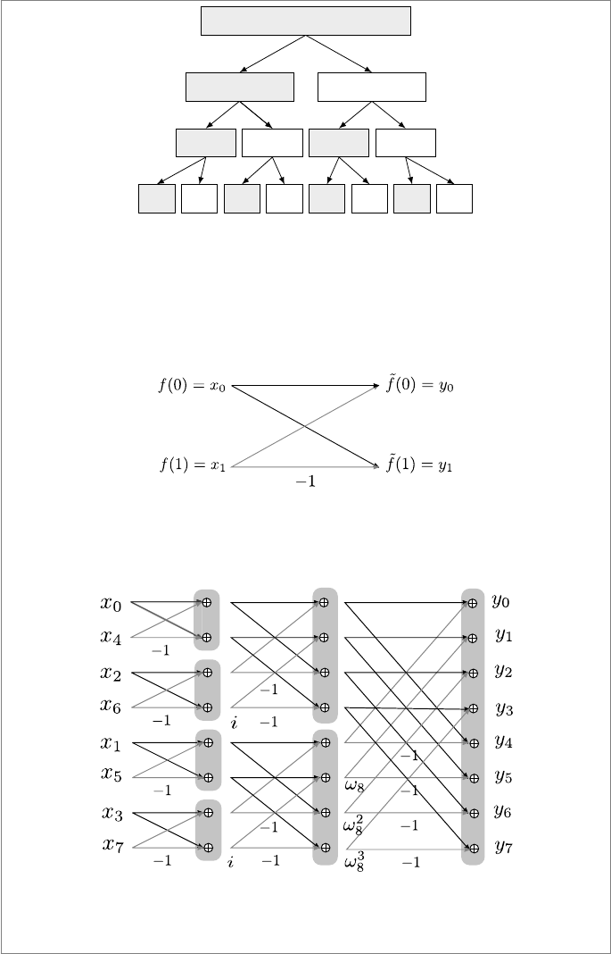
Successive division of the terms in the input into two until we reach the
two-term pairs is called decimation. The process of decimating higher-order
DFT’s looks like the following for N = 8:
Quantum Algorithms 157
x
0
x
1
x
2
x
3
x
4
x
5
x
6
x
7
x
0
x
2
x
4
x
6
x
1
x
3
x
5
x
7
x
0
x
4
x
2
x
6
x
1
x
5
x
3
x
7
x
0
x
4
x
2
x
6
x
1
x
5
x
3
x
7
even
odd
We then start evaluating upward from the 2-point DFTs, successively dou-
bling at each stage. The generic 2-point DFT looks like Figure 8.8, called a
butterfly diagram for its symmetric structure. The labels on the sides represent
the multiplicative factors and two lines joined at a node represent addition of
the corresponding terms.
FIGURE 8.8: The 2-point DFT: butterfly diagram.
For N = 8, we have worked out the decimation process in Example 8.4.4.
The butterfly diagram looks like Figure 8.9.
FIGURE 8.9: Butterfly diagram for computing an 8-point DFT.
The output vector {y
0
y
1
. . . y
8
} is the DFT of the input vector.
Leave a Reply