
Even though the Bernstein–Vazirani algorithm offers such a great speedup,
the classical solution is still not exponential. Daniel Simon came up with an
algorithm [65] in 1994 that is the first to demonstrate a dramatic exponential
speedup over a hard classical problem, but the solution is probabilistic. This
feature is characteristic of many quantum algorithms. Simon’s problem also
illustrates a class of problems that basically use Fourier transforms, in the
form of the amplitudes of the output states that “interfere” to give a large
probability for the expected solution.
The problem: Given a black box implementing a function
f : {0, 1}
n
7→ {0, 1}
n−1
such thatf(x ⊕ a) = f(x), a ∈ [0, 2
n
− 1], (8.15)
determine a with the minimum number of queries to the box.
Example 8.3.1. The functions considered in Simon’s algorithm can be thought
of as “periodic” under bitwise addition. For example, let’s look at the 3-bit
function
x 000 001 010 011 100 101 110 111
f(x) 3 2 2 3 1 4 4 1
The first repetition is of the value f(1) = f(2). The “period” is therefore
a = 001 ⊕ 010 = 011 = 3. You can verify that all the other repetitions also
satisfy the same condition.
Quantum Algorithms 151
The classical solution to this problem is hard, i.e., the number of runs
of the function grows exponentially as the size of the input. We would query
the oracle with successive values of n-bit numbers x until we found a repeated
value for the output: f (x
i
) = f (x
j
). Then we could calculate a = x
i
⊕ x
j
.
However, a could be any one of 2
n
possible numbers. By the m
th
run,
1
2
m(m−
1) pairs have been compared and eliminated as possible a’s. For reasonable
chance of success, we need
1
2
m(m−1) ≥ 2
n
=⇒ a lower bound on the number
of trials m = Ω(2
n/2
), which is exponential in the number of bits.
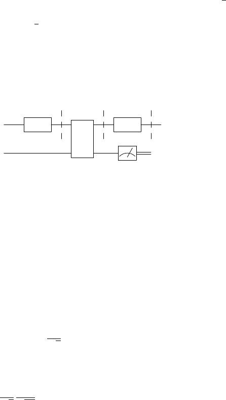
The quantum circuit (Figure 8.7) that solves this problem is essentially
the same as the Deutsch–Josza circuit except that the lower register is also
expanded to n qubit, and initialized to |0i
n
(we dispense with the phase
kickback).
|ψ
0
i |ψ
1
i |ψ
2
i
|0i
n
/
n
H
⊗n
/
n
U
f
H
⊗n
/
n
|0i
n
/
n
f(x
0
)
FIGURE 8.7: The circuit for the Simon algorithm.
The input to the oracle gives us
U
f
|ψ
0
i ⊗ |0i = U
f
“
2
n
−1
X
x=0
|xi ⊗ |0i
#
=
2
n
−1
X
x=0
|xi ⊗ |f(x)i. (8.16)
In order to analyze the solution, let us use the reverse of the principle of
delayed measurement, and assume we measure the lower register after the
action of U
f
. Let’s denote the outcome by f (x
0
), which is generated from
two possible inputs x
0
or x
0
⊕ a. The top register therefore collapses to a
superposition of these two states alone:
|ψ
1
i =
1
√
2
(|x
0
i + |x
0
⊕ ai) . (8.17)
If we now apply H to each qubit in the upper register, we get
|ψ
3
i =
1
√
2
1
√
2
n
2
n
−1
X
y=0
h
(−1)
x
0
·y
+ (−1)
(x
0
⊕a)·y
i
|yi. (8.18)
Now a · y is either 0 or 1. If a · y = 1, then the amplitude for |yi is zero and
all those states do not occur in the output. Thus the only states that can be
measured in the output are those for which the condition a ·y = 0 is satisfied.
This is a binary algebraic equation with n unknowns (the bits of a). We can
find a if we can obtain n independent equations, corresponding to n different
values of y. If we repeat the experiment until we have collected n distinct,
152 Introduction to Quantum Physics and Information Processing
non-zero y’s then we can solve for the bits of a. It is not guaranteed that we
will get a distinct y on each run, so we may most probably have to run the
oracle more than n times.
To determine the complexity of this problem, we will need to estimate
how the number of runs of the oracle scales with n. It can be shown (see Box
8.3) that the number of times the oracle has to be queried is n + m where m
doesn’t depend on n. This algorithm is thus a sub-exponential solution to a
classically hard problem.
Box 8.1: Complexity Analysis for Simon’s Algorithm
As in many quantum algorithms, the analysis of why the algorithm is com-
putationally more efficient than the classical case involves a detailed math-
ematical examination of the solution. In the case of Simon’s algorithm, the
output after measurement is an n-bit string y such that
a · y = a
n−1
y
n−1
⊕ a
n−2
y
n−2
⊕ ··· ⊕ a
1
y
1
⊕ a
0
y
0
= 0.
We need to collect at least n −1 such distinct bit-strings in order to determine
the coefficients a. So we need to query the oracle at least n −1 times and need
to find a lower bound on the probability of success.
Suppose we ran the algorithm k times and got linearly independent y’s.
What’s the probability that the next run gives a different y? The minimum
probability for this occurring is
2
n
− 2
k
2
n
= 1 − 2
k−n
.
So the probability of getting n − 1 independent y’s is just
P =
1 −
1
2
n
1 −
1
2
n−1
. . .
1 −
1
2
.
Now notice that (1 − s)(1 − t) = 1 − (s + t) + st ≥ 1 − (s + t). So we have
P ≥
1 −
n
X
i=1
1
2
i
!
1
2
≥
1 −
1
2
1
2
=
1
4
.
This means that there is a finite minimum probability with which we will
succeed in n runs. To ensure success, we’ll have to run the algorithm a few
more times, independent of n, so that the number of runs is still O(n).
The trick that makes the kind of algorithms considered so far work is that
the output before measuring in the X basis has f(x)-dependent phases.
Leave a Reply