
We’ll now look at algorithms that show more substantial speedups com-
pared to classical ones. One such algorithm was invented by Umesh Vazirani
and his student Ethan Bernstein in 1993 [11]. This algorithm identifies a linear
Boolean function in one query of the oracle.
The problem: given a function evaluator for
f : {0, 1}
n
7→ {0, 1} where f (x) = a · x, a ∈ [0, 2
n
], (8.11)
and the dot is a bitwise product with modulo 2 addition:
a · x ≡ a
0
x
0
⊕ a
1
x
1
⊕ ··· ⊕ a
n−1
x
n−1
, (8.12)
determine the function, or in other words find a.
Example 8.2.1. An example of such a function for n = 2 and a = 11, which
evaluates to
f(00) = 0
Quantum Algorithms 149
f(01) = 0.1 ⊕ 1.1 = 1
f(10) = 1.1 ⊕ 0.1 = 1
f(11) = 1.1 ⊕ 1.1 = 0
Classically, we can determine the k
th
bit of a if we feed the oracle the
input x = 2
k
, that has only the k
th
bit as 1 and all the rest as 0. This becomes
obvious when you look at the binary expansion of a:
a = a
0
+ a
1
2
1
+ ··· + a
k
2
k
+ . . . =⇒ a
k
= a · 2
k
. (8.13)
This calls the function n times.
The quantum algorithm, which uses the same circuit as for the
Deutsch–Josza algorithm, succeeds with one call!
Let’s analyze the output of the circuit of Figure 8.4 for this form of the
function:
X
x
X
y
1
2
n
(−1)
f(x)+x·y
|yi ⊗ |−i =
1
2
n
X
y
“
X
x
(−1)
a·x+y·x
#
|yi ⊗ |−i
. (8.14)
The amplitude for |yi is
1
2
n
P
x
(−1)
a·x+y·x
=
1
2
n
P
x
(−1)
(a+y)·x
= 1 if
y = a! It’s easy to see why it is zero for all other values of y. Thus with
certainty, the output of the circuit gives us a.
A more explicit way of seeing why this works is by analyzing the circuit for
U
f
. This analysis is lucidly given in Mermin [48]. The black box for a·x flips the
bit in the lower register whenever a bit of the input x and the corresponding
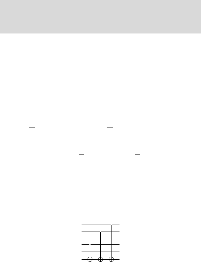
bit of a are both 1. For instance, suppose we had a = 11010 with n = 5. Then
it can easily be seen that a · x is implemented by the circuit of Figure 8.5.
a = 11010
x
4
•
x
3
•
x
2
x
1
•
x
0
|0i |a · xi
FIGURE 8.5: A circuit that executes U
f
for f = 11010 · x.
Coming to the circuit for solving the Bernstein–Vazirani problem, it has
an H gate before each qubit enters the function evaluator and after. This is
true even of the lower register, which can be thought of as initialized to |1i.
Note that an H gate before and after a CNOT interchanges the roles of the
control and target qubits (see Figure 7.8).
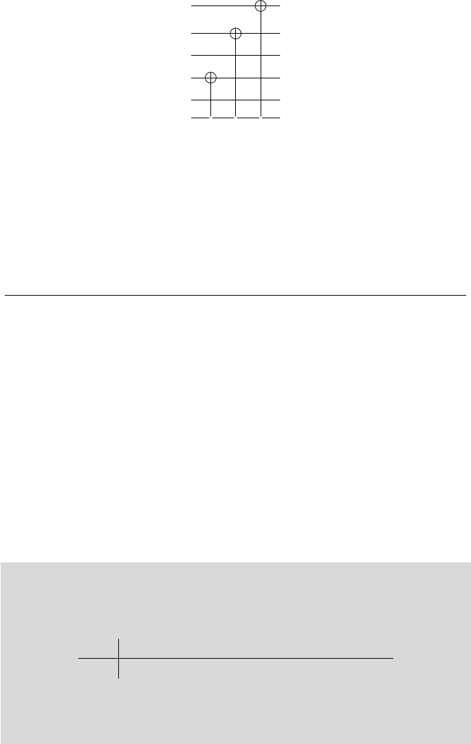
150 Introduction to Quantum Physics and Information Processing
|0i |1i
|0i |1i
|0i |0i
|0i |1i
|0i |0i
|1i
• • •
FIGURE 8.6: Analysis of circuit for the Bernstein–Vazirani algorithm for a =
11010.
The solution is therefore the circuit of Figure 8.6, whose output directly
reads out the bits of a.
The algorithm thus gives an n-fold speedup over the classical case
Leave a Reply