
As mentioned previously, one of the major responsibilities of a chemical engineer involves determination of power and energy requirements for the flow of fluids. This requires understanding the energy balance for the fluid flow, presented in section 5.2.1.
5.2.1 Energy Balance for Fluid Flow
The energy balance for systems involving a simple flow of a fluid is characterized by the lack of conversion of chemical, thermal, or any other kind of energy into mechanical energy. Essentially, the resulting mathematical formulation is simply a mechanical energy balance wherein the energy contributions arise from the potential and kinetic energy terms and flow work [3]. For an incompressible (constant density) fluid that does not experience any friction, the mechanical energy balance is given by equation 5.1 [1]:
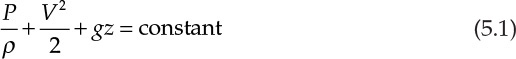
where P is the pressure, V is the velocity, ρ is the density of the fluid, and z is the elevation of the fluid in the gravitational field, g being the acceleration due to gravity. The terms in the equation have the units of J/kg (energy per unit mass), and this equation is known as the Bernoulli equation [1]. The validity of the Bernoulli equation is limited to frictionless flow, but in reality, frictional effects need to be accounted for. Applying the Bernoulli equation between points 1 and 2 yields equation 5.2 [1]:
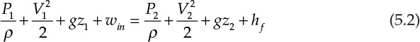
where hf represents the frictional losses. It is assumed that the fluid flow is accomplished by means of a pump between the two points, and win is simply the work input from this pump. It should be clear from equation 5.2 that the power requirement for transferring a fluid from one point to another depends on the following four factors:2
2. A student will encounter the detailed analysis while conducting the mechanical energy balance in later curriculum.
• The difference in the hydrostatic pressure between the two points
• The difference in the elevation of the two points
• The difference between the fluid velocities at the two points
• The frictional losses in the piping system
The frictional losses depend on the flow regime, and the accounting of the frictional losses requires an understanding of the concept of viscosity.
5.2.2 Viscosity
The concept of friction is easily understood for a rigid, solid object. For a solid object to move, it must overcome the resistance from another object in contact with it. A similar situation can be envisioned in the case of a flowing fluid. Consider the velocity profile for laminar flow shown in Figure 5.2. The molecules are flowing in layers stacked upon each other. The molecules in contact with the wall can be considered to be stationary because of friction with the wall—a state called the no-slip condition. The layer of molecules adjoining this layer has to slide against this stationary layer. Similarly, there is relative motion between all adjacent layers, causing frictional losses. The resistance to motion between the layers is highest at the wall, decreasing toward the center of the conduit.
This variation in axial velocity with the position in the direction normal to the flow direction causes a shear stress in the fluid. This shear stress multiplied by the area over which it enacts yields the shear force—the frictional resistance to the flow. The shear stress for a fluid depends on the velocity gradient—how rapidly the velocity changes with distance. The following shows this mathematically [4]:
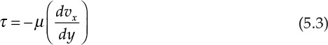
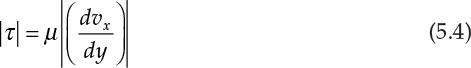
where τ is the shear stress, and vx the velocity in the x-direction, which depends on the position in the y-direction. Equation 5.3, known as Newton’s law of viscosity, indicates that the shear stress is directly proportional to the velocity gradient, with the constant of proportionality being μ, which is the dynamic viscosity of the fluid. Fluids that follow this simple relationship are termed Newtonian fluids. Many other fluids not conforming to this relationship are termed non-Newtonian. The negative sign in the equation arises from the directional considerations, with velocity and position being vector quantities, viscosity being a scalar, and the shear stress a tensor. The directional considerations are disregarded in the calculations in this book, and only absolute values are considered, reducing the equation to the following form:
The SI unit of viscosity is N·s/m2 (equivalently, Pa·s or kg/m·s), the centimeter-gram-second (CGS) system unit being poise (P or g/cm·s). Viscosity is a function of temperature, the viscosity of water being 1 cP or 1 mPa·s at ~21°C. In contrast, viscosities of honey and glycerin are between 1500 and 2000 cP at ambient temperatures. The difficulty with which these fluids flow can be explained on the basis of their viscosities. Viscosities of substances can be predicted from theory or experimentally determined.
The force needed for getting the liquid to flow can be obtained by multiplying the shear stress with the area over which it acts, which is the contact surface area between the layers. The pressure differential needed to make the fluid flow can then be obtained by dividing the force by the cross-sectional flow area, which is the area in the direction perpendicular to the flow direction.
5.2.3 Reynolds Number
As previously mentioned, the flow regime is laminar at low flow rates. Frictional viscous forces predominate at these flow rates. As the flow rate increases, the orderly laminar arrangement is disrupted and the inertial forces associated with the movement of material begin to predominate. The ratio of these two forces can be related to the intrinsic fluid properties (viscosity µ, density ρ) and flow parameters (characteristics length dimension l, average velocity v) through a dimensionless quantity termed Reynolds number in honor of Osborne Reynolds:

Reynolds, in his experiments, observed that the transition from laminar to turbulent flow occurred at the Reynolds number of 2300; that is, the flow was laminar below this value and began transitioning into turbulent flow above it. This transition may take place over a range of Reynolds numbers, the flow often considered to be fully turbulent when Re exceeds 4000. The characteristic length dimension depends on the system geometry. For cylindrical conduits, diameter d is used as the length dimension for calculating Re. It should be noted that these Re ranges are applicable to internal flows, that is, a flow through conduits. For external flows, that is, flows over surfaces and objects, such as flow around a car or an airplane, other quantitative criteria apply for the laminar to turbulent transition [5].
5.2.4 Pressure Drop Across a Flow Conduit
The frictional losses due to the flow of fluids result in a decrease of pressure from the point upstream to the point downstream. In other words, a higher upstream pressure is needed to overcome frictional losses in order to transfer fluid from the point upstream to the point downstream. The pressure drop can be viewed as the potential that induces fluid flow, analogous to voltage in an electrical circuit. Different mathematical expressions are used to obtain this pressure drop for the two different flow regimes.
The following equation shows the pressure drop for laminar flow through a pipe with constant circular cross section of diameter d:
In this equation, ΔP is the pressure drop over pipe length L when the volumetric flow rate is Q. Equation 5.6 is called the Hagen-Poiseuille equation [1] in honor of G. Hagen and J. L. Poiseuille, who developed this formulation.
For turbulent flow, the pressure drop is given by the following:
where f is the friction factor3, which is a function of the Reynolds number. Figure 5.3 shows the generalized trend exhibited by the friction factor as a function of the Reynolds number [3]. The friction factor, in the turbulent regimes, also shows a dependence on the roughness of the pipe, as indicated by the value of the parameter k/D in the figure.
3. The friction factor, as used here and by chemical engineers generally, is the Fanning friction factor. Mechanical and civil engineers often use the Darcy friction factor, which, while calculated differently, has the same physical significance.
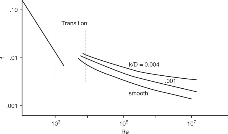
Figure 5.3 A generalized friction factor plot.
Source: Thomson, W. J., Introduction to Transport Phenomena, Prentice Hall, Upper Saddle River, New Jersey, 2000.
Chemical engineers often use the Nikuradse equation (covered in Chapter 4, “Introduction to Computations in Chemical Engineering”) for calculating the friction factor for turbulent flow through smooth pipes:
This equation is valid for flows having Re between 4000 and 3.2 × 10⁶. The pressure drop so obtained is used further in the mechanical energy balance equation to calculate the power requirements for pumping the fluid.
Leave a Reply