Prediction via Equations

You can see from Figure 7.2 (line AB) that the function of p* versus T is not a linear function (except as an approximation over a very small temperature range). Many functional forms have been proposed to predict p* from T, but we use the Antoine equation in this text because it has sufficient accuracy for our needs, and coefficients for the equation exist in the literature for over 5000 compounds:ln(p*)=A−BC+T

(7.4)

where A, B, C = constants for each substance, and T = temperature, kelvin.

Refer to Appendix F (available online; see Preface, page xvi) for the values of A, B, and C for various compounds.

You can estimate the values of A, B, and C in Equation (7.4) from experimental data by using a regression program such as found in MATLAB and Python. With just three experimental values for the vapor pressure versus temperature, you can fit Equation (7.4), but more values are better!

Example 7.2 Vaporization of Metals for Thin Film Deposition

Problem Statement

Three methods of providing vaporized metals for thin film deposition are evaporation from a boat, evaporation from a filament, and transfer via an electronic beam. Figure E7.2 illustrates evaporation from a boat placed in a vacuum chamber.

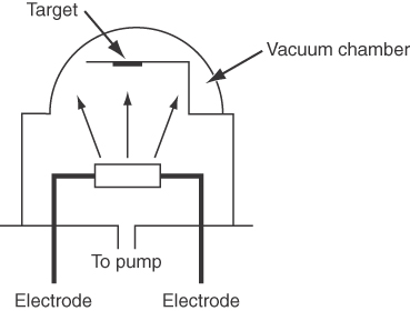
The boat made of tungsten has a negligible vapor pressure at 972°C, the operating temperature for the vaporization of aluminum (which melts at 660°C and fills the boat). The approximate rate of evaporation m is given in g/(cm²)(s) bym=0.437p*(MW)1/2T1/2

where p* is the vapor pressure in kilopascals, MW is the molecular weight and T is the temperature in kelvin. What is the vaporization rate for Al at 972°C in g/(cm²)(s)?

Solution

You have to calculate p* for Al at 972°C. The Antoine equation is suitable if data are known for the vapor pressure of Al. Considerable variation exists in the data for Al at high temperatures, but we will use A = 8.779, B = 1.615 × 104, and C = 0 with p* in millimeters of Hg and T in kelvin.In p972°C*=8.799−1.615×104972+273=0.0154 mm Hg (0.00201 kPa)m=0.437(0.00201)(26.98)1/2(972+273)1/2=1.3×10−4 g/(cm2)(s)

7.3.2 Retrieving Vapor Pressures from the Tables

You can find the vapor pressures of substances listed in tables in handbooks, physical property books, and websites. We use water as an example. Tabulations of the properties of water and steam (water vapor) are commonly called the steam tables, although the tables are as much about water as they are about steam. The properties of water and steam from one source may not agree precisely with other sources because the values available from different sources are likely generated by using equations having different accuracy and precision.

Four classes of tables exist in the foldout:

1. A table of p* versus T (saturated water and vapor) listing other properties such as V^Properties of Saturated WaterVolume, m³/kgPress. kPaT (K)V^_lV_g0.80276.920.001000159.71.0280.130.001000129.21.2282.810.001000108.71.4285.130.00100193.921.6287.170.00100182.761.8288.990.00100174.032.0290.650.00100267.002.5294.230.00100254.253.0297.230.00100345.674.0302.120.00100434.80
2. A table of T versus p* (saturated water and vapor) containing other properties such as V^Properties of Saturated WaterVolume (m³/kg)T (K)Press. (kPa)V^_lV_g273.160.61130.001000206.12750.69800.001000181.72800.99120.001000130.32851.3880.00100194.672901.9190.00100169.672952.6200.00100251.903003.5360.00100439.103054.7180.00100529.783106.2300.00100722.913158.1430.00100917.80
3. A table listing superheated vapor (steam) properties as a function of T and pSuperheated Steam^*Abs. Press. lb/in.² (Sat. Temp. °F)Sat. WaterSat. Steam400°F420°F440°FSh29.2349.2369.23175v0.01822.6012.7302.8142.897(370.77)h343.611196.71215.61227.61239.9Sh26.9246.9266.92180v0.01832.5322.6482.7312.812(373.08)h346.071197.21214.61226.81239.2Sh24.6644.6664.66185v0.01832.4662.5702.6512.731(375.34)h348.471197.61213.71226.01238.4^*Sh = degrees of superheat, °F; v = specific volume, ft³/lb_m; h = specific enthalpy, Btu/lb_m
4. A table of subcooled water (liquid) properties as a function of p and T (h and u in this table are the specific enthalpy and the specific internal energy, respectively, which are introduced in Chapter 8)Properties of Liquid Waterp, kPa400425450Sat.ρ, kg/m³937.35915.08890.25h, kJ/kg532.69639.71748.98u, kJ/kg532.43639.17747.93500ρ, kg/m³937.51915.08h, kJ/kg532.82639.71u, kJ/kg532.29639.17700ρ, kg/m³937.62915.22h, kJ/kg532.94639.84u, kJ/kg532.19639.07

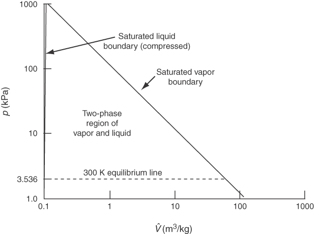
Locate each table in the foldout, and use the tables with the following explanations. How can you tell which table to use to get the properties you want? One way is to look at one of the phase diagrams for water. For example, do the conditions of 25°C and 4 atm refer to liquid water, a saturated liquid-vapor mixture, or water vapor? You can use the values in the steam tables plus what you know about phases to reach a decision about the state of the water. In the SI steam tables of T versus p* for saturated water, T is just less than 300 K at which p* = 3.536 kPa. Because the given pressure was about 400 kPa, much higher than the saturation pressure at 298 K, clearly the water is subcooled (compressed liquid).

Can you locate the point p* = 250 kPa and V^=1.00 m3/kg using Figure 7.8? Do you find the water is in the superheated steam region? The specified volume is larger than the saturated volume of 0.7187 m³/kg at 250 kPa. What about the point T = 300 K and V^=0.505  m3/kg? Water at that state is a mixture of saturated liquid and vapor. You can calculate the quality of the water-water vapor mixture using Equation (7.1) as follows: From the steam tables, the specific volumes of the saturated liquid and vapor are

V^l=0.001004  m3/kg   V^g=39.10 m3/kgBasis: 1 kg of wet  steam mixture

Let x = mass fraction vapor. Then0.001004 m31 kg liquid|(1−x)kg liquid+39.10 m31 kg vapor|x kg vapor=0.505 m3                                   x=0.0129 (the fractional quality)

If you are given a specific mass of saturated water plus steam at a specified temperature or pressure so that you know the state of the water is in the two-phase region, you can use the steam tables for various calculations. For example, suppose a 10.0 m³ vessel contains 2000 kg of water plus steam at 10 atm, and you are asked to calculate the volume of each phase. Let the volume of water be V_l and the volume of steam be Vg; then the masses of each phase are Vl/V^l and Vg/V^g respectively. From your knowledge of the total volume and total mass:

V_l + V_g = 10

andVl/V^l+Vg/V^g=2000

From the steam tables, V^l=0.0011274  m3/kg and V^g=0.19430  m3/kg. Solving these simultaneous equations for V_l and V_g gives the volume of the liquid as 2.21 m³ and the volume of the steam as 7.79 m³. The mass of the liquid is 1960 kg, and the mass of the steam is 40 kg.

Because the values in the steam tables are tabulated in discrete increments, for intermediate values, you will have to interpolate to retrieve values between the discrete values. (If interpolation does not appeal to you, use the physical property software on the website that accompanies this book.) The next example shows how to carry out interpolations in tables.

Example 7.3 Interpolating in the Steam Tables

Problem Statement

What is the saturation pressure of water at 312 K?

Solution

To solve this problem, you have to carry out a single interpolation. Look in the steam tables under the properties of saturated water to get p* so as to bracket 312 K:T(K)p*(kPa)3106.2303158.143

Figure E7.3 shows the concept of a linear interpolation between 310 K and 315 K. Find the change of p* per unit change in T.

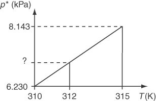
Δp*ΔT=8.143−6.230315−310=1.915=0.383

Multiply the fractional change times the number of degrees increase from 310 K to get change in p*, and add the result to the value of p* at 310 K of 6.230 kPa:p312 K*=p310 K*+Δp*ΔT(T312−T310)=6.230+0. 383(2)=7.000 kPa

7.3.3 Predicting Vapor Pressures from Reference Substance Plots

Because of the curvature of the vapor-pressure data versus temperature (see Figure 7.2), no simple equation with two or three coefficients will fit the data accurately from the triple point to the critical point. Othmer proposed in numerous articles¹ that reference substance plots (the name will become clear in a moment) could convert the vapor-pressure-versus-temperature curve into a straight line. One well-known example is the Cox chart.² You can use the Cox chart to retrieve vapor-pressure values as well as to test the reliability of experimental data, to interpolate, and to extrapolate. Figure 7.9 is a Cox chart.

¹ See, for example, D. F. Othmer, Ind. Eng. Chem., 32, 841 (1940); and J. H. Perry and E. R. Smith, Ind. Eng. Chem., 25, 195 (1933).

² E. R. Cox, Ind. Eng. Chem., 15, 592 (1923).

Here is how you can make a Cox chart:

1. Mark on the horizontal scale values of log p* so as to cover the desired range of p*.
2. Next, draw a straight line on the plot at a suitable angle, say, 45°, that covers the range of T that is to be marked on the vertical axis.
3. To calibrate the vertical axis in common integers such as 25, 50, 100, 200 degrees, and so on, you use a reference substance, usually water. For the first integer, say, T = 100°F, you look up the vapor pressure of water in the steam tables, or calculate it from the Antoine equation, to get 0.9487 psia. Locate this value on the horizontal axis, and proceed vertically until you hit the 45° straight line. Then proceed horizontally left until you hit the vertical axis. Mark the scale there as 100°F.
4. Pick the next temperature, say, 200°F, and get 11.525 psia. Proceed vertically from p* = 11.525 to the 45° straight line, and then horizontally to the vertical axis. Mark the scale as 200°F.
5. Continue as in steps 3 and 4 until the vertical scale is established over the desired range for the temperature.

Other compounds will give straight lines for p* versus T as shown in Figure 7.9. What proves useful about the Cox chart is that the vapor pressures of other substances plotted on this specially prepared set of coordinates will yield straight lines over extensive temperature ranges and thus facilitate the extrapolation and interpolation of vapor-pressure data. It has been found that lines so constructed for closely related compounds, such as hydrocarbons, all meet at a common point. Since straight lines can be obtained in a Cox chart, only two points of vapor-pressure data are needed to provide adequate information about the vapor pressure of a substance over a considerable temperature range.

Let’s look at an example of using a Cox chart.

Example 7.4 Extrapolation of Vapor-Pressure Data

Problem Statement

The control of solvents was first described in the Federal Register [36, No. 158 ( August 14, 1971)] under Title 42, Chapter 4, Appendix 4.0, “Control of Organic Compound Emissions.” Chlorinated solvents and many other solvents used in industrial finishing and processing, dry-cleaning plants, metal degreasing, printing operations, and so forth can be recycled and reused by the introduction of carbon adsorption equipment. To predict the size of the adsorber, you first need to know the vapor pressure of the compound being adsorbed at the process conditions.

The vapor pressure of chlorobenzene is 400 mm Hg absolute at 110°C and 5 atm at 205°C. Estimate the vapor pressure at 245°C and also at the critical point (359°C).

Solution

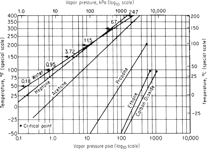
The vapor pressures will be estimated by use of a Cox chart. You construct the temperature scale (vertical) and vapor-pressure scale (horizontal) as described in connection with Figure 7.9. On the horizontal axis with p* given in a log₁₀ scale, mark the vapor pressures of water from 3.72 to 3094 psia corresponding to 150°F to 700°F, and mark the respective temperatures on the vertical scale as shown in Figure E7.4.

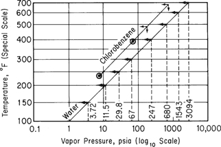
Next, convert the two given vapor pressures of chlorobenzene into psia:400   mm  Hg  |14.7 psia760 mm Hg=7.74 psia 110°C=230° F5 atm|14.7 psia1 atm=73.5 psia 205°C=401° F

and plot these two points on the graph paper. Examine the encircled dots. Finally, draw a straight line between the encircled points and extrapolate to 471°F (245°C) and 678°F (359°C). At these two temperatures, you can read off the estimated vapor pressures.

	471°F (245°C)	678° (359°C)
Estimated:	150 psia	700 psia
Experimental:	147 psia	666 psia

Experimental values are given for comparison.

7.3.4 Using MATLAB and Python to Interpolate Nonlinear Data

Linear interpolation can be highly accurate when applied to certain data sets and not so accurate for other. How can you tell if a set of data lends itself to linear interpolation or requires nonlinear interpolation? The following two data sets can be used to address this issue:

Vapor Pressure and Specific Volume of Liquid Saturated Steam
T (K)	Vapor Pressure (kpa)	dpvpdT	V^lip(m3/kg)×104	dV^lipdT×104
275	0.6980	0.059	9.9959	0.0013
280	0.9912	0.059	10.0022	0.0012
285	1.388	0.079	10.0084	0.0012
290	1.919	0.106	10.0147	0.0012
295	2.620	0.140	10.0209	0.0019
300	3.536	0.183	10.0334	0.0025
305	4.718	0.236	10.0459	0.0037
310	6.230	0.302	10.0709	0.0044
315	8.143	0.383	10.0896	0.0037

The data sets come from the saturated steam data for the vapor pressure and the specific volume of liquid water as functions of temperature. For nonlinear data, the slope of the data changes significantly, while for relatively linear data, the slope changes gradually. Also, when you plot the data on a linear scale, the plot will have significant curvature for a nonlinear set of data. Note that the derivatives of the vapor pressure with respect to temperature changes by a factor of 6 for the range of temperatures shown, while the specific volume of the liquid changed by a factor of 3. Therefore, both sets of data contain significant nonlinearity.

Now note that the total change in the specific volume for this set of data is less than 1% while the total change for the vapor pressure is about 250%. Therefore, the relative change in the specific volume between data points is quite small. As a result, linear interpolation applied to the data for the specific volume will provide highly accurate approximations of the data. On the other hand, the relative change between data for the vapor pressure is significant. Therefore, the combination of the nonlinearity of the data and the magnitude of relative change between adjacent data values for the vapor pressure will produce significant error if linear interpolation is used. This point is demonstrated by the following two examples.

Both MATLAB and Python offer functions that apply interpolation based on a cubic spline approximating equation. A spline is a nonlinear function that can be viewed as a mathematical representation of a flexible curve because the function will pass through each data point but can have slopes that vary through the data set. The following examples demonstrate how to apply these cubic spline functions for interpolation of data that cannot be accurately interpolated using linear interpolation.

MATLAB

MATLAB offers a built-in function for cubic spline interpolation: function spline. The call statement for function spline is given by

fv=spline(xd,fd,xv)

where fv is the interpolated value based on xv, xd is a vector containing the values of x for the data used for the interpolation, fd is a vector containing the values of f(x) for the data used for the interpolation, and xv is the value of x used for the interpolation. Function spline uses linear, quadratic, or cubic interpolation depending on the nonlinearity of the data.

Example 7.5 Cubic Spline Interpolation Using MATLAB

Problem Statement

Using the saturated steam data for vapor pressure in the last table, estimate the vapor pressure at 307.5 K.

Solution

MATLAB Solution for Example 7.5

Click here to view code image%%%%%%%%%%%%%%%%%%%%%%%%%%%%%%%%%%%%%%%%%%%%%%%%%%%%%%%%%%%%%% % NOMENCLATURE % % fv – the interpolated value % xd – a vector containing the x values of the data % fd – a vector containing the y values of the data % xv- the value of x that is to be interpolated % %%%%%%%%%%%%%%%%%%%%%%%%%%%%%%%%%%%%%%%%%%%%%%%%%%%%%%%%%%%%%% % PROGRAMfunction Ex7_5_Splineclear; clc; % Insert data xd=[275,280,285,290,295,300,305,310,315];fd=[0.6968,0.9912,1.388,1.919,2.62,3.536,4.718,6.23,8.143];xv=[307.5]; % Set value to be interpolated fv=spline(xd,fd,xv) % Call built-in function spline end % PROGRAM END %%%%%%%%%%%%%%%%%%%%%%%%%%%%%%%%%%%%%%%%%%%%%%%%%%%%%%%%%%%%%%% fv = 5.4284

Analysis of Results. If linear interpolation were used for this example, the result would be 5.474 kPa, and this amounts to a difference of 0.046 kPa between linear and cubic spline interpolation, which is a relatively small difference but nevertheless significant based on the number of digits reported in the vapor pressure data.

Python

Python offers a built-in function for interpolation: scipy.interpolate.interp1d. The call statement for interp1d is given by

f=scipy.interpolate.interp1d(xd, yd, kind=’linear’)

yi=f(xv)

where f is a function that can be used for interpolation, xd is a vector containing the values of x for the data used for the interpolation, yd is a vector containing the values of y(x) for the data used for the interpolation, xv is the value of x for which interpolation evaluation is to be made, and yi is the interpolated value for xv. scipy.interpolate.interp1d offers linear, quadratic, or cubic spline interpolation depending on the value of kind for which the default is linear (i.e., 'linear', 'quadratic', or 'cubic'). Note that function f determined by this function can be used for a single interpolation or for a number of interpolations.

Example 7.6 Cubic Spline Interpolation Using Python

Problem Statement

Using the saturated steam data for vapor pressure in the last table, estimate the vapor pressure at 307.5 K.

Solution

Python Code for Example 7.6

Click here to view code imageEx7_6 Interpolation.py ######################################################################### # NOMENCLATURE # # xd – a vector containing the x values for the data # xv- a vector containing the values of x that are to be used for interpolation # yd – a vector containing the y values for the data # yi – the interpolated value ######################################################################### # PROGRAMimport scipy.interpolateimport numpy as np # Input the x,y data xd=np.array([275, 280, 285, 290, 295, 300, 305, 310, 315])yd=np.array([0.6968, 0.9912, 1.388, 1.919, 2.62, 3.536, 4.718, 6.23, 8.143]) # # Apply function scipy.interpolate.interp1d to implement cubic spine interpolation # f=scipy.interpolate.interp1d(xd, yd, kind=‘cubic’) # Specify the value that will be used to perform the interpolation xv=307.5 # Use the function determined by scipy.interpolate.interp1d to perform the interpolation yi=f(xv)print(“The interpolated value for x={0:5.2f} is {1:6.4f}”.format(xv, yi)) # PROGRAM END #########################################################################

IPython Console:

Click here to view code image In[1]: runfile(… Out[1]: The interpolated value for x=307.5 is 5.4284 kPa

Analysis of Results. If linear interpolation were used for this example, the result would be 5.474 kPa, and this amounts to a difference of 0.046 kPa between linear and cubic spline interpolation, which is a relatively small difference but nevertheless significant based on the number of digits reported in the vapor pressure data.

Although this chapter uses the vapor pressure of a pure component, we should mention that the term vapor pressure has been applied to solutions of multiple components as well. For example, to meet emission standards, refiners formulate gasoline and diesel fuel differently in the summer than in the winter. The rules on emissions are related to the vapor pressure of a fuel, which is specified in terms of the Reid vapor pressure (RVP), a value that is determined at 100°F in a bomb that permits partial vaporization. For a pure component, the RVP is the true vapor pressure, but for a mixture (as are most fuels), the RVP is lower than the true vapor pressure of the mixture (by roughly 10% for gasoline).³

³ Refer to J. J. Vazquez-Esparragoza, G. A. Iglesias-Silva, M. W. Hlavinka, and J. Bulin, “How to Estimate RVP of Blends,” Hydrocarbon Processing, 135 (August, 1992), for specific details about estimating the RVP.