Introducing the Effects of Mixing into the Energy Balance

In Section 12.1 we restricted the discussion and examples to the standard state (25°C and 1 atm). In this section we proceed with what happens when the temperatures of the inlet and outlet streams differ from 25°C for a binary mixture in an open, steady-state process. (For a closed system the initial and final states of the internal energy would be involved rather than the stream flows.) You can treat problems involving the heat of solution/mixing in exactly the same way that you can treat problems involving reaction. The heat of solution/mixing is analogous to the heat of reaction in the energy balance. You can carry out the needed calculations by

1. a. Associating heats of formation of the compounds and solutions with each of the respective compounds and solutions, or
2. b. Computing the overall lumped heat of solution at the reference state, and for either option calculating the sensible heats (and phase change effects) for the compounds and solutions from the reference state.

The next example shows the detailed procedure.

Example 12.2 Application of Heat of Solution Data

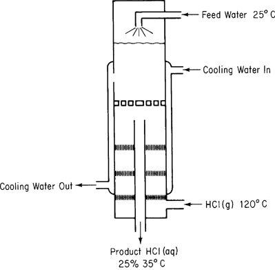
Hydrochloric acid is an important industrial chemical. To make aqueous solutions of it in a commercial grade (known as muriatic acid), purified HCl(g) is absorbed in water in a tantalum absorber in a steady-state continuous process. How much heat must be removed from the absorber by the cooling water per 100 kg of product if hot HCl(g) at 120°C is fed into water in the absorber as shown in Figure E12.2? The feed water can be assumed to be at 25°C, and the exit product HCl(aq) is 25% HCl (by weight) at 35°C. The cooling water does not mix with the HCl solution.

Solution

Steps 1–4

You need to convert the process data to moles of HCl to be able to use the data in Table 12.1. Consequently, we will first convert the product into moles of HCl and moles of H₂O.

Table E12.2a

Component		kg	Mol. wt.	kg mol	Mole Fraction
HCl		25	36.37	0.685	0.141
H2O		75	18.02	4.163	0.859
	Total	100		4.848	1.000

The mole ratio of H₂O to HCl is 4.163/0.685 =6.077.

Step 5

The system will be the HCl and water (not including the cooling water).

Basis: 100 kg of product

Ref. temperature: 25°C

Steps 6 and 7

The energy balance reduces to Q = ΔH, and both the initial and final enthalpies of all of the streams are known or can be calculated directly; hence the problem has zero degrees of freedom. From simple material balances the kilograms and moles of HCl in and out, and the water in and out, are as listed in Table E12.2a above.

Step 3 (continued)

Next, you have to determine the enthalpy values for the streams. Data are: C_p for the HCl(g) is from Table G.1; C_p for the product is approximately 2.7 J/(g)(°C) equivalent to 55.6 J/(g mol) (°C); ΔH^Fo for HCl · 6.077 H₂O ≌ −157,753 J/g mol HCl. We will use ΔH^Fo values for each stream in the calculation of ΔH.

Steps 8 and 9

Table E12.2b

Stream		g mol	T(°C)	ΔH^fo(J/g molHCl)	ΔH^sensible(J/gmol)
OUT
	HCl (aq)	4.848*	35	−157,753	∫25°C35°C(2.7)dT
IN
	H2O(l)	4.163	25	−
	HCl(g)	0.685	120	−92,311	∫25°C120°C(29.13−0.134×10−2T)dT   =2758

^*HCl=0.685Q=ΔHout−ΔHinOut                                                                             In=[0.685(−157,753)+4.848(27)]−[0+0.685(−92,311)+0.685(2758)]=−46,586J

If you use heat of solution values, the calculation is (from Table 12.1 the heat of solution is −65,442 J/g mol HCl for the ratio of HCl/H₂O =6.077)Q=ΔHout,sensible−ΔHin,sensible+ΔHsensible=(4.848)(27)−[0.685(2753)+0]+(0.685)(−65,442)=−46,586⁢ J      as expected

In a process simulation code, table lookup or equations would be used to calculate the heats of formation at various temperatures (and pressures) other than 25°C (and 1 atm). The details would be buried in the computer code. You can better understand what the calculations for an energy balance involve if you use a graph—at the expense of some accuracy—instead of equations.

A convenient graphical way to represent enthalpy data for binary solutions is via an enthalpy-concentration diagram. Enthalpy-concentration diagrams (H-x) are plots of specific enthalpy versus concentration (usually mass or mole fraction) with temperature as a parameter. Figure 12.3 illustrates one such plot. If available,¹ such charts are useful in making combined material and energy balance calculations in distillation, crystallization, and all sorts of mixing and separation problems. You will find a few examples of enthalpy-concentration charts in Appendix J.

¹For a literature survey as of 1957, see Robert Lemlich, Chad Gottschlich, and Ronald Hoke, Chem. Eng. Data Ser., 2 , 32 (1957). Additional references: for CC1₄, see M. M. Krishniah et al, J. Chem. Eng. Data, 10 , 117 (1965); for EtOH-EtAc, see Robert Lemlich, Chad Gottschlich, and Ronald Hoke, Br. Chem. Eng., 10 , 703 (1965); for methanol-toluene, see C. A. Plank and D. E. Burke, Hydrocarbon Process, 45 , No. 8, 167 (1966); for acetone-isopropanol, see S. N. Balasubramanian, Br. Chem. Eng., 12 , 1231 (1967); for acetonitrile-water-ethanol, see Reddy and Murti, ibid., 13 , 1443 (1968); for alcohol-aliphatics, see Reddy and Murti, ibid., 16 , 1036 (1971); and for H₂SO₄, see D. D. Huxtable and D. R. Poole, Proc. Int. Solar Energy Soc., Winnipeg, August 15, 1976, 8 , 178 (1977). For more recent sources search the Internet.

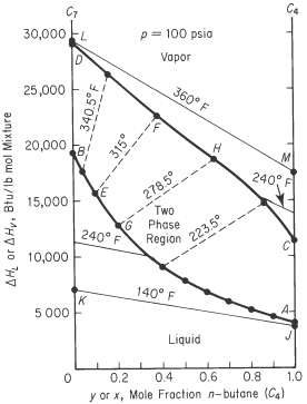
As you might expect, the preparation of an enthalpy-concentration chart requires numerous calculations and valid enthalpy or heat capacity data for solutions of various concentrations. Refer to Unit Operations of Chemical Engineering [W. L. McCabe and J. C. Smith, 3rd ed., McGraw-Hill, New York (1976)] for instructions if you have to prepare such a chart. In the next example we show how to use an H-x chart.

Example 12.3 Application of an Enthalpy-Concentration Chart

Six hundred pounds of 10% NaOH per hour at 200°F are added to 400 lb/hr of 50% NaOH at the boiling point in an insulated vessel. Calculate the following:

1. a. The final temperature of the exit solution
2. b. The final concentration of the exit solution
3. c. The pounds of water evaporated per hour during the process

Solution

You can use the steam tables and the NaOH-H₂O enthalpy-concentration chart in Appendix J as your sources of data. What are the reference conditions for the chart? The reference conditions for the latter chart are ΔH^Fo = 0 at 32°F for pure liquid water, an infinitely dilute solution of NaOH. Pure caustic has an enthalpy at 68°F of 455 Btu/lb above this datum. Treat the process as a flow process even if is not. The energy balance reduces to ΔH=0. Basis: 1000 lb of final solution =1 hr.

You can write the following material balances:

Component	10% solution	+	50% solution	=	Final solution	wt%
NaOH	60		200		260	26
H2O	540		200		740	74
Total	600		400		1000	100

Enthalpy data from the H-x chart

ΔH^(Btu/lb): 10% solution 152 50% solution 290

The energy balance is

10% solution		50% solution		Final solution
600(152)	+	400(290)	=	ΔH
91,200	+	116,000	=	207,200

Note that the enthalpy of the 50% solution at its boiling point is taken from the bubble point at ω_NaOH = 0.50. The enthalpy per pound of the final solution is207,200Btu1000lb=207 Btu/lb

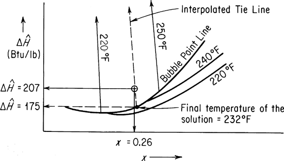
On the enthalpy-concentration chart for NaOH-H₂O, for a 26% NaOH solution with an enthalpy of 207 Btu/lb, you would find that only a two-phase mixture of (1) saturated H₂O vapor and (2) NaOH-H₂O solution at the boiling point could exist. To get the fraction H₂O vapor, you have to make an additional energy (enthalpy) balance. By interpolation, draw the tie line through the point x=0.26, H=207 (make it parallel to the 220°F and 250°F tie lines). The final temperature of the tie line appears from Figure E12.3 to be 232°F; the enthalpy of the liquid at the bubble point at this temperature is about 175 Btu/lb. The enthalpy of the saturated water vapor (no NaOH is in the vapor phase) from the steam tables at 232°F is 1158 Btu/lb. Let x=pounds of H₂O evaporated.

Basis: 1000 lb of final solution

x(1158) +(1000 −x) 175 = 1000 (207.2)

x = 32.8 of H₂O evaporated/hr