
Many important processes involve the adsorption of gases or liquids on solids. Some examples for liquids are
- Decolorizing, drying, or “degumming” of petroleum fractions
- Odor, taste, and color removal from municipal water supplies
- Decolorizing of vegetable and animal oils, and of crude sugar syrups
- Clarification of beverages and pharmaceutical preparations
- Purification of process effluents and gases for pollution control
- Solvent recovery from air such as in removing evaporated dry-cleaning solvents
- Dehydration of gases
- Odor and toxic gas removal from air or vent gases
- Separation of rare gases at low temperatures
- Impurity removal from air prior to low-temperature fractionation
- Storage of hydrogen
What goes on in adsorption? Adsorption is a physical phenomenon that occurs when gas or liquid molecules are brought into contact with a solid surface, the adsorbent. Some of the molecules may condense (the adsorbate) on the exterior surface and in the cracks and pores of the solid. If interaction between the solid and condensed molecules is relatively weak, the process is called physical adsorption; if the interaction is strong (similar to a chemical reaction), it is called chemisorption, or activated adsorption. We focus on equilibria in physical adsorption in this chapter.
Equilibrium adsorption is analogous to the gas-liquid and liquid-liquid equilibria described in previous chapters. Picture a small section of adsorbent surface. As soon as molecules come near the surface, some condense on the surface. A typical molecule will reside on the adsorbent for some finite time before it acquires sufficient energy to leave. Given sufficient time, an equilibrium state will be reached: The number of molecules leaving the surface will just equal the number arriving.
The number of molecules on the surface at equilibrium is a function of the (1) nature of the solid adsorbent, (2) nature of the molecule being adsorbed (the adsorbate), (3) temperature of the system, and (4) concentration of the adsorbate over the adsorbent surface. Numerous theories have been proposed to relate the amount of fluid adsorbed to the amount of adsorbent. The various theories lead to equations that represent the equilibrium state of the adsorption system. Theoretical models hypothesize various physical conditions such as (1) a solid surface on which there is a monomolecular layer of molecules, or (2) a multimolecular layer, or (3) capillary condensation.
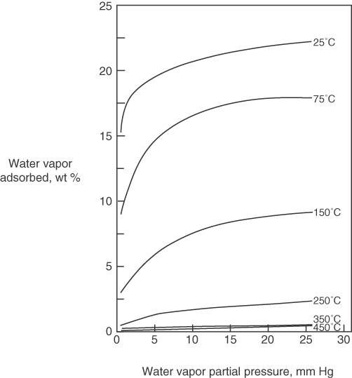
Figure 13.1 illustrates typical simple equilibrium adsorption isotherms for the adsorption of water vapor on Type 5A molecular sieves at various temperatures. Note how the amount of gas adsorbed decreases as the temperature increases.
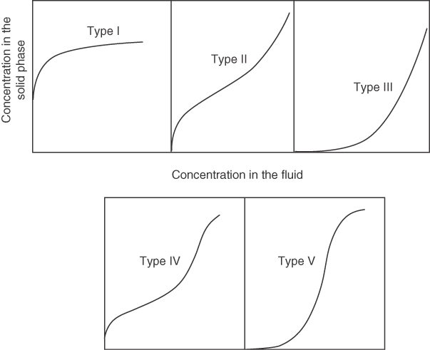
No single relation can represent all of the myriad types of equilibrium data found in practice, as indicated by the variety of curves for isothermal adsorption called adsorption isotherms, shown in Figure 13.2.
Two of the simpler equilibrium relations for physical adsorption of Type I in Figure 13.2 relate the amount adsorbed for a single component (the adsorbate) on the adsorbent as a function of the adsorbate partial pressure in the gas phase, or the concentration in the liquid phase, at some temperature. These equations apply for low concentrations at equilibrium.
Freundlich Isotherm
| For a gas: | For a liquid: |
| y=k1pn1 | y=k2xn2 |
where p is the partial pressure of the adsorbate in the gas phase
y is the cumulative mass of solute or gas adsorbed (adsorbate) per mass of adsorbent in the solid phase
x is the mass of solute per mass of solution in the liquid phase
ni and ki are coefficients
Langmuir Isotherm
| For a gas: | For a liquid: |
| y=(1+ak3)p1+k3p | y=(1+bk4)x1+k4x |
The respective equations correspond to monolayer adsorption. Numerous other relations have been developed to match the particular shapes of the adsorption equilibrium data shown in Figure 13.2. Refer to the references at the end of this chapter.
You can obtain values for the coefficients in the equilibrium isotherms by fitting them to experimental data, as shown in Example 13.1. The expressions (1 + ak3) and (1 + bk4) can be treated as single coefficients in the fitting.
Example 13.1 Fitting Adsorption Isotherms to Experimental Data
The following data for the adsorption of CO2 on 5A molecular sieves at 298 K have been taken from the PhD dissertation Periodic Countercurrent Operation of Pressure-Swing Adsorption Processes Applied to Gas Separations by Carol L. Blaney [University of Delaware (1985), p. 131].
| p CO2 (mm Hg) | y (g adsorbed/g sieves) |
|---|---|
| 0 | 0 |
| 25 | 6.69 × 10⁻² |
| 50 | 9.24 × 10⁻² |
| 100 | 0.108 |
| 200 | 0.114 |
| 400 | 0.127 |
| 760 | 0.137 |
The estimated coefficients in the respective isotherms obtained by using the regression function in Polymath 5 were:
| Freundlich Isotherm | Langmuir Isotherm | ||||
|---|---|---|---|---|---|
| Model: y + apn | R2 = 0.993 | Model: ap /(1 + bp) | R2 = 0.981 | ||
| Variable | Initial guess | Final value | Variable | Initial guess | Final value |
| a | 1 | 0.0448 | a | 100 | 0.0052 |
| n | 0.5 | 0.1729 | b | 1 | 0.0386 |
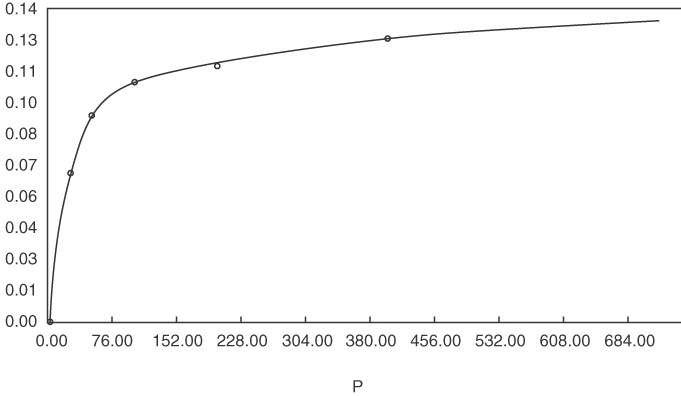
The parameter R2 is a measure of the degree of fit; R2 = 1 is a perfect fit. Figure E13.1 shows the data and the adsorption isotherms.
A type of constant that is used in environmental studies is the soil sorption partition coefficient, Koc. It characterizes the partitioning of a compound between the solid and liquid phases in soil, and is used to determine the mobility of a compound in soil:
Koc=μg of compound adsorbed g of organic carbon in the soil μg of compound in the liquid phase mL liquid in the liquid phase
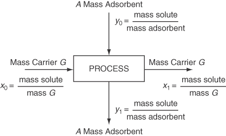
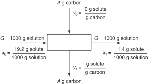
How do you use the information about adsorption in practice? One way is to combine it with material balances to help design adsorption equipment. Examine Figure 13.3 in which a carrier G (gas or liquid) is contacted with an adsorbent A (solid). Assume that the vessel is well mixed and that the exit streams are in equilibrium with each other.
The mass of G is the mass of the carrier excluding the solute, and the mass of A is also solute free. Often we assume the solution entering is dilute enough so that G is equivalent to the total flow. The material balance corresponding to the process in Figure 13.3 is (note that x and y are not mass fractions in what follows)lnG(x0−x1)=OutA(y1−y0)
(13.1)
Usually the A entering is free of solute so that y0 = 0, and thus the material balance becomesG(x0−x1)=Ay1
(13.2)
Example 13.2 shows how the Freundlich isotherm can be combined with a material balance to solve a design problem.
Example 13.2 Combination of an Adsorption Isotherm with a Material Balance
You are asked to calculate the minimum mass of activated carbon required to reduce a contaminating solute in a fermentation system from x0 = 19.2 g solute/L solution (for simplicity the value can be treated as grams of solute per 1000 g solution) to x1 = 1.4 g solute/L solution for a 1 L batch of solution by adsorption on activated charcoal in a well-mixed vessel so that the output products are in equilibrium. To solve this problem you collect the following liquid-solid equilibria data. Note that the third column contains calculated, not measured, values.
| Measured at equilibrium | ||
|---|---|---|
| Cumulative g Carbon Added per 1000 g Solution | x g Solute | y (Calculated) g Solute Adsorbed |
| 1000 g Solution | g Carbon | |
| 0 | 19.2 | — |
| 0.01 | 17.2 | (19.2–17.2)/0.01 = 200 |
| 0.04 | 12.6 | (19.2–12.6)/0.04 = 165 |
| 0.08 | 8.6 | (19.2–8.6)/0.08 = 133 |
| 0.20 | 3.4 | (19.2–3.4)/0.20 = 79 |
| 0.40 | 1.4 | (19.2–1.4)/0.40 = 45 |
Solution
Steps 1–4
If you fit the data using Polymath, the Freundlich isotherm proves to bey=37.919 x0.583 R2=0.999
(a)
and the Langmuir isotherm isy=(29.698x)/(1+0.0955x) R2=0.987
(b)
Figure E13.2, the process diagram, shows the flows in and out of the system. From a different viewpoint, the process is equivalent to a batch process in which the materials are put into an empty vessel at the start and removed at the end of the process. Let G be the grams of solution. Because the solution is so dilute, G is essentially equivalent to the grams of solute-free solvent. If you wanted to, you could calculate the ratios of the solute to the solute-free solvent coming in and out of the process, but we will not do so.
Step 5
Let the basis be 1000 g solution (1 L).
Steps 6–9
Two independent equations are involved in the solution, an equilibrium relation and the material balance. Two unknowns exist, y1 and the ratio A/G.
Combine Equation (a) with Equation (13.2) to get
AG=x0−x1y1=(19.2−1.4)g solute 1000g solution 37.919(1.4)0.583g solute g carbon =17.846.1=0.39g carbon 1000g solution
Hence, 0.39 g carbon is required.
Step 10
You can check the answer by using the Langmuir isotherm together with the material balance:
AG=19.2−1.4Y1
y1=29.698(1.4)1+0.0955(1.4) or y1 = 36.67
hence
AG=17.836.67=0.48 g carbon/1000 g solution
Because y1 = 46.1 from the Freundlich isotherm is closer to the experimental value of 45 than is 36.7 from the Langmuir isotherm, the value of 0.39 g as the answer would be preferred. Of course, more carbon will have to be used in practice because to reach equilibrium takes a very long time.
Can you now calculate how much carbon would be required to remove all of the polluting solute?
Leave a Reply