
The earth makes one rotation about its axis every 24 h and completes a revolution about the sun in a period of approximately 365.25 days. This revolution is not circular but follows an ellipse with the sun at one of the foci, as shown in Figure 2.3. The eccentricity, e, of the earth’s orbit is very small, equal to 0.01673. Therefore, the orbit of the earth round the sun is almost circular. The sun–earth distance, R, at perihelion (shortest distance, at January 3) and aphelion (longest distance, at July 4) is given by Garg (1982):
![]() (2.4)
(2.4)
where a = mean sun–earth distance = 149.5985 × 10⁶ km.
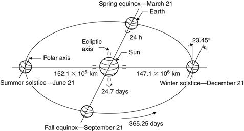
FIGURE 2.3 Annual motion of the earth about the sun.
The plus sign in Eq (2.4) is for the sun–earth distance when the earth is at the aphelion position and the minus sign for the perihelion position. The solution of Eq (2.4) gives values for the longest distance equal to 152.1 × 10⁶ km and for the shortest distance equal to 147.1 × 10⁶ km, as shown in Figure 2.3. The difference between the two distances is only 3.3%. The mean sun–earth distance, a, is defined as half the sum of the perihelion and aphelion distances.
The sun’s position in the sky changes from day to day and from hour to hour. It is common knowledge that the sun is higher in the sky in the summer than in winter. The relative motions of the sun and earth are not simple, but they are systematic and thus predictable. Once a year, the earth moves around the sun in an orbit that is elliptical in shape. As the earth makes its yearly revolution around the sun, it rotates every 24 h about its axis, which is tilted at an angle of 23° 27.14 min (23.45°) to the plane of the elliptic, which contains the earth’s orbital plane and the sun’s equator, as shown in Figure 2.3.
The most obvious apparent motion of the sun is that it moves daily in an arc across the sky, reaching its highest point at midday. As winter becomes spring and then summer, the sunrise and sunset points move gradually northward along the horizon. In the Northern Hemisphere, the days get longer as the sun rises earlier and sets later each day and the sun’s path gets higher in the sky. On June 21 the sun is at its most northerly position with respect to the earth. This is called the summer solstice and during this day the daytime is at a maximum. Six months later, on December 21, the winter solstice, the reverse is true and the sun is at its most southerly position (see Figure 2.4). In the middle of the 6-month range, on March 21 and September 21, the length of the day is equal to the length of the night. These are called spring and fall equinoxes, respectively. The summer and winter solstices are the opposite in the Southern Hemisphere; that is, summer solstice is on December 21 and winter solstice is on June 21. It should be noted that all these dates are approximate and that there are small variations (difference of a few days) from year to year.
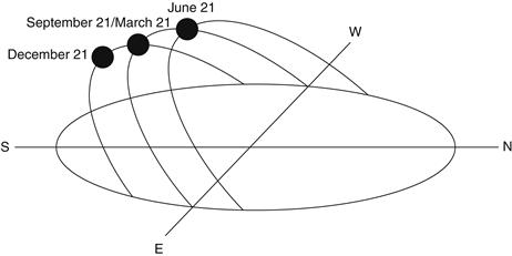
FIGURE 2.4 Annual changes in the sun’s position in the sky (Northern Hemisphere).
For the purposes of this book, the Ptolemaic view of the sun’s motion is used in the analysis that follows, for simplicity; that is, since all motion is relative, it is convenient to consider the earth fixed and to describe the sun’s virtual motion in a coordinate system fixed to the earth with its origin at the site of interest.
For most solar energy applications, one needs reasonably accurate predictions of where the sun will be in the sky at a given time of day and year. In the Ptolemaic sense, the sun is constrained to move with 2 degrees of freedom on the celestial sphere; therefore, its position with respect to an observer on earth can be fully described by means of two astronomical angles, the solar altitude (α) and the solar azimuth (z). The following is a description of each angle, together with the associated formulation. An approximate method for calculating these angles is by means of sun path diagrams (see Section 2.2.2).
Before giving the equations of solar altitude and azimuth angles, the solar declination and hour angle need to be defined. These are required in all other solar angle formulations.
Declination, δ
As shown in Figure 2.3 the earth axis of rotation (the polar axis) is always inclined at an angle of 23.45° from the ecliptic axis, which is normal to the ecliptic plane. The ecliptic plane is the plane of orbit of the earth around the sun. As the earth rotates around the sun it is as if the polar axis is moving with respect to the sun. The solar declination is the angular distance of the sun’s rays north (or south) of the equator, north declination designated as positive. As shown in Figure 2.5 it is the angle between the sun–earth centerline and the projection of this line on the equatorial plane. Declinations north of the equator (summer in the Northern Hemisphere) are positive, and those south are negative. Figure 2.6 shows the declination during the equinoxes and the solstices. As can be seen, the declination ranges from 0° at the spring equinox to +23.45° at the summer solstice, 0° at the fall equinox, and −23.45° at the winter solstice.
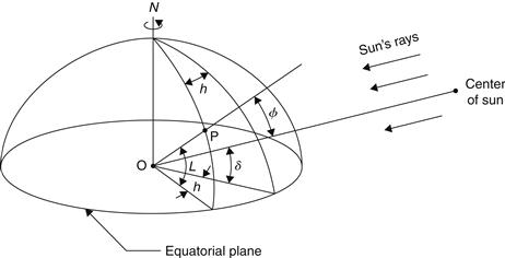
FIGURE 2.5 Definition of latitude, hour angle, and solar declination.
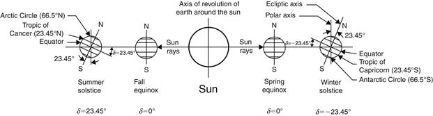
FIGURE 2.6 Yearly variation of solar declination.
The variation of the solar declination throughout the year is shown in Figure 2.7. The declination, δ, in degrees for any day of the year (N) can be calculated approximately by the equation (ASHRAE, 2007):
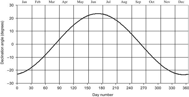
FIGURE 2.7 Declination of the sun.
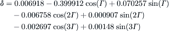
Declination can also be given in radians1 by the Spencer formula (Spencer, 1971):
 (2.6)
(2.6)
where Γ is called the day angle, given (in radians) by:
![]() (2.7)
(2.7)
The solar declination during any given day can be considered constant in engineering calculations (Kreith and Kreider, 1978; Duffie and Beckman, 1991).
As shown in Figure 2.6, the Tropics of Cancer (23.45°N) and Capricorn (23.45°S) are the latitudes where the sun is overhead during summer and winter solstices, respectively. Another two latitudes of interest are the Arctic (66.5°N) and Antarctic (66.5°S) Circles. As shown in Figure 2.6, at winter solstice all points north of the Arctic Circle are in complete darkness, whereas all points south of the Antarctic Circle receive continuous sunlight. The opposite is true for the summer solstice. During spring and fall equinoxes, the North and South Poles are equidistant from the sun and daytime is equal to nighttime, both of which equal 12 h.
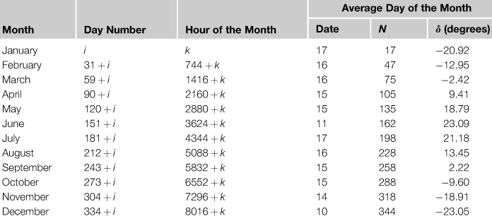
Because the day number, the hour of the month, and the average day of each month are frequently required in solar geometry calculations, Table 2.1 is given for easy reference.
Table 2.1
Day Number and Recommended Average Day for Each Month
Hour angle, h
The hour angle, h, of a point on the earth’s surface is defined as the angle through which the earth would turn to bring the meridian of the point directly under the sun. Figure 2.5 shows the hour angle of point P as the angle measured on the earth’s equatorial plane between the projection of OP and the projection of the sun–earth center to center line. The hour angle at local solar noon is zero, with each 360/24 or 15° of longitude equivalent to 1 h, afternoon hours being designated as positive. Expressed symbolically, the hour angle in degrees is:
![]() (2.8)
(2.8)
where the plus sign applies to afternoon hours and the minus sign to morning hours.
The hour angle can also be obtained from the AST; that is, the corrected local solar time:
![]() (2.9)
(2.9)
At local solar noon, AST = 12 and h = 0°. Therefore, from Eq (2.3), the LST (the time shown by our clocks at local solar noon) is:
![]() (2.10)
(2.10)
EXAMPLE 2.2
Find the equation for LST at local solar noon for Nicosia, Cyprus.
Solution
For the location of Nicosia, Cyprus, from Example 2.1,

EXAMPLE 2.3
Calculate the apparent solar time on March 10 at 2:30 pm for the city of Athens, Greece (23°40′E longitude).
Solution
The ET for March 10 (N = 69) is calculated from Eq (2.1), in which the factor B is obtained from Eq (2.2) as:


Therefore,

The standard meridian for Athens is 30°E longitude. Therefore, the AST at 2:30 pm, from Eq (2.3), is:

Solar altitude angle, α
The solar altitude angle is the angle between the sun’s rays and a horizontal plane, as shown in Figure 2.8. It is related to the solar zenith angle, Φ, which is the angle between the sun’s rays and the vertical. Therefore,
![]() (2.11)
(2.11)
The mathematical expression for the solar altitude angle is:
![]() (2.12)
(2.12)
where L = local latitude, defined as the angle between a line from the center of the earth to the site of interest and the equatorial plane. Values north of the equator are positive and those south are negative.
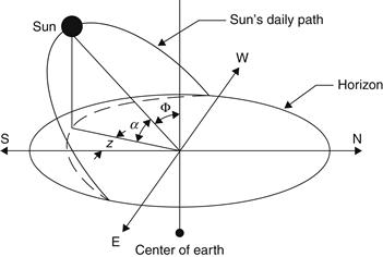
FIGURE 2.8 Apparent daily path of the sun across the sky from sunrise to sunset.
Solar azimuth angle, z
The solar azimuth angle, z, is the angle of the sun’s rays measured in the horizontal plane from due south (true south) for the Northern Hemisphere or due north for the Southern Hemisphere; westward is designated as positive. The mathematical expression for the solar azimuth angle is:
![]() (2.13)
(2.13)
This equation is correct, provided that cos(h) > tan(δ)/tan(L) (ASHRAE, 1975). If not, it means that the sun is behind the E–W line, as shown in Figure 2.4, and the azimuth angle for the morning hours is −π + |z| and for the afternoon hours is π − z.
At solar noon, by definition, the sun is exactly on the meridian, which contains the north–south line, and consequently, the solar azimuth is 0°. Therefore the noon altitude αn is:
EXAMPLE 2.4
What are the maximum and minimum noon altitude angles for a location at 40° latitude?
Solution
The maximum angle is at summer solstice, where δ is maximum, that is, 23.5°. Therefore, the maximum noon altitude angle is 90°− 40° + 23.5° = 73.5°.
The minimum noon altitude angle is at winter solstice, where δ is minimum, that is, −23.5°. Therefore, the minimum noon altitude angle is 90° − 40° − 23.5° = 26.5°.
Sunrise and sunset times and day length
The sun is said to rise and set when the solar altitude angle is 0. So, the hour angle at sunset, hss, can be found by solving Eq. (2.12) for h when α = 0°:

or
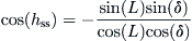
which reduces to:
![]() (2.15)
(2.15)
where hss is taken as positive at sunset.
Since the hour angle at local solar noon is 0°, with each 15° of longitude equivalent to 1 h, the sunrise and sunset time in hours from local solar noon is then:
![]() (2.16)
(2.16)
The sunrise and sunset hour angles for various latitudes are shown in Figure A3.1 in Appendix 3.
The day length is twice the sunset hour, since the solar noon is at the middle of the sunrise and sunset hours. Therefore, the length of the day in hours is:
![]() (2.17)
(2.17)
EXAMPLE 2.5
Find the equation for sunset standard time for Nicosia, Cyprus.
Solution
The LST at sunset for the location of Nicosia, Cyprus, from Example 2.1 is:

EXAMPLE 2.6
Find the solar altitude and azimuth angles at 2 h after local noon on June 16 for a city located at 40°N latitude. Also find the sunrise and sunset hours and the day length.
Solution
From Eq. (2.5), the declination on June 16 (N = 167) is:
From Eq. (2.8), the hour angle, 2 h after local solar noon is:
From Eq. (2.12), the solar altitude angle is:

Therefore,

From Eq. (2.13), the solar azimuth angle is:
Therefore,

From Eq. (2.17), the day length is:

This means that the sun rises at 12 − 7.4 = 4.6 = 4:36 am solar time and sets at 7.4 = 7:24 pm solar time.
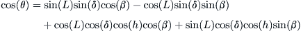
Incidence angle, θ
The solar incidence angle, θ, is the angle between the sun’s rays and the normal on a surface. For a horizontal plane, the incidence angle, θ, and the zenith angle, Φ, are the same. The angles shown in Figure 2.9 are related to the basic angles, shown in Figure 2.5, with the following general expression for the angle of incidence (Kreith and Kreider, 1978; Duffie and Beckman, 1991):
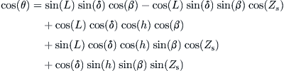 (2.18)
β = surface tilt angle from the horizontal,
Zs = surface azimuth angle, the angle between the normal to the surface from true south, westward is designated as positive.
For certain cases Eq. (2.18) reduces to much simpler forms:
• For horizontal surfaces, β = 0° and θ = Φ, and Eq. (2.18) reduces to Eq. (2.12).
• For vertical surfaces, β = 90° and Eq. (2.18) becomes:
![]() (2.19)
(2.19)
• For a south-facing tilted surface in the Northern Hemisphere, Zs = 0° and Eq. (2.18) reduces to:
which can be further reduced to:
![]() (2.20)
(2.20)
• For a north-facing tilted surface in the Southern Hemisphere, Zs = 180° and Eq. (2.18) reduces to:
![]() (2.21)
(2.21)
Equation (2.18) is a general relationship for the angle of incidence on a surface of any orientation. As shown in Eqs (2.19)–(2.21), it can be reduced to much simpler forms for specific cases.
EXAMPLE 2.7
A surface tilted 45° from horizontal and pointed 10° west of due south is located at 35°N latitude. Calculate the incident angle at 2 h after local noon on June 16.
Solution
From Example 2.6 we have δ = 23.35° and the hour angle = 30°. The solar incidence angle θ is calculated from Eq. (2.18):
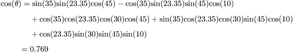
Therefore,

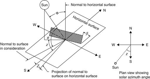
FIGURE 2.9 Solar angles diagram.
The incidence angle for moving surfaces
For the case of solar-concentrating collectors, some form of tracking mechanism is usually employed to enable the collector to follow the sun. This is done with varying degrees of accuracy and modes of tracking, as indicated in Figure 2.10.
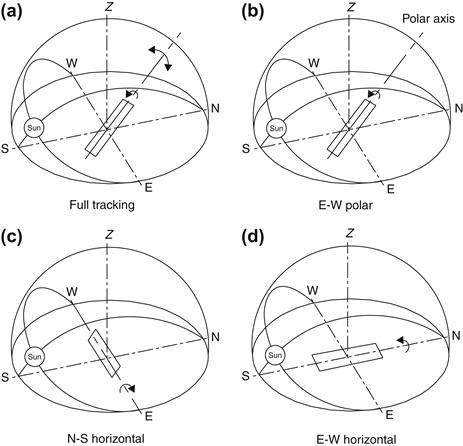
FIGURE 2.10 Collector geometry for various modes of tracking.
Tracking systems can be classified by the mode of their motion. This can be about a single axis or about two axes (Figure 2.10(a)). In the case of a single-axis mode, the motion can be in various ways: parallel to the earth’s axis (Figure 2.10(b)), north–south (Figure 2.10(c)), or east–west (Figure 2.10(d)). The following equations are derived from the general Eq. (2.18) and apply to planes moved, as indicated in each case. The amount of energy falling on a surface per unit area for the summer and winter solstices and the equinoxes for latitude of 35°N is investigated for each mode. This analysis has been performed with a radiation model. This is affected by the incidence angle, which is different for each mode. The type of model used here is not important, since it is used for comparison purposes only.
Full tracking
For a two-axis tracking mechanism, keeping the surface in question continuously oriented to face the sun (see Figure 2.10(a)) at all times has an angle of incidence, θ, equal to:
![]() (2.22)
(2.22)
or θ = 0°. This, of course, depends on the accuracy of the mechanism. The full tracking configuration collects the maximum possible sunshine. The performance of this mode of tracking with respect to the amount of radiation collected during one day under standard conditions is shown in Figure 2.11.
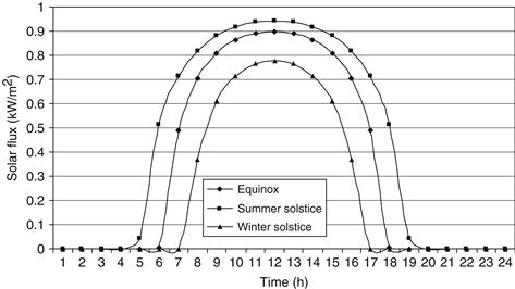
FIGURE 2.11 Daily variation of solar flux, full tracking.
The slope of this surface (β) is equal to the solar zenith angle (Φ), and the surface azimuth angle (Zs) is equal to the solar azimuth angle (z).
Tilted N–S axis with tilt adjusted daily
For a plane moved about a north–south axis with a single daily adjustment so that its surface normal coincides with the solar beam at noon each day, θ is equal to (Meinel and Meinel, 1976; Duffie and Beckman, 1991):
![]() (2.23)
(2.23)
For this mode of tracking, we can accept that, when the sun is at noon, the angle of the sun’s rays and the normal to the collector can be up to a 4° declination, since for small angles cos(4°) = 0.998 ∼ 1. Figure 2.12 shows the number of consecutive days that the sun remains within this 4° “declination window” at noon. As can be seen in Figure 2.12, most of the time the sun remains close to either the summer solstice or the winter solstice, moving rapidly between the two extremes. For nearly 70 consecutive days, the sun is within 4° of an extreme position, spending only 9 days in the 4° window, at the equinox. This means that a seasonally tilted collector needs to be adjusted only occasionally.
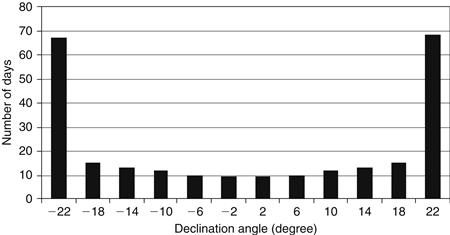
FIGURE 2.12 Number of consecutive days the sun remains within 4° declination.
The problem encountered with this and all tilted collectors, when more than one collector is used, is that the front collectors cast shadows on adjacent ones. Therefore, in terms of land utilization, these collectors lose some of their benefits when the cost of land is taken into account. The performance of this mode of tracking (see Figure 2.13) shows the peaked curves typical for this assembly.
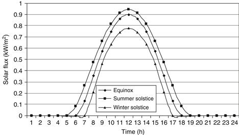
FIGURE 2.13 Daily variation of solar flux: tilted N–S axis with tilt adjusted daily.
Polar N–S axis with E–W tracking
For a plane rotated about a north–south axis parallel to the earth’s axis, with continuous adjustment, θ is equal to:
![]() (2.24)
(2.24)
This configuration is shown in Figure 2.10(b). As can be seen, the collector axis is tilted at the polar axis, which is equal to the local latitude. For this arrangement, the sun is normal to the collector at equinoxes (δ = 0°) and the cosine effect is maximum at the solstices. The same comments about the tilting of the collector and shadowing effects apply here as in the previous configuration. The performance of this mount is shown in Figure 2.14.
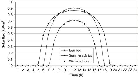
FIGURE 2.14 Daily variation of solar flux: polar N–S axis with E–W tracking.
The equinox and summer solstice performance, in terms of solar radiation collected, are essentially equal; that is, the smaller air mass for summer solstice offsets the small cosine projection effect. The winter noon value, however, is reduced because these two effects combine. If it is desired to increase the winter performance, an inclination higher than the local latitude would be required; but the physical height of such configuration would be a potential penalty to be traded off in cost-effectiveness with the structure of the polar mount. Another side effect of increased inclination is shadowing by the adjacent collectors, for multi-row installations.
The slope of the surface varies continuously and is given by:
![]() (2.25a)
(2.25a)
The surface azimuth angle is given by:
![]() (2.25b)
(2.25b)
where
![]() (2.25c)
(2.25c)
 (2.25d)
![]() (2.25e)
(2.25e)
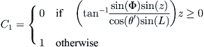
Horizontal E–W axis with N–S tracking
For a plane rotated about a horizontal east–west axis with continuous adjustment to minimize theangle of incidence, θ can be obtained from (Kreith and Kreider, 1978; Duffie and Beckman, 1991):
![]() (2.26a)
(2.26a)
or from this equation (Meinel and Meinel, 1976):
![]() (2.26b)
(2.26b)
The basic geometry of this configuration is shown in Figure 2.10(c). The shadowing effects of this arrangement are minimal. The principal shadowing is caused when the collector is tipped to a maximum degree south (δ = −23.5°) at winter solstice. In this case, the sun casts a shadow toward the collector at the north. This assembly has an advantage in that it approximates the full tracking collector in summer (see Figure 2.15), but the cosine effect in winter greatly reduces its effectiveness. This mount yields a rather “square” profile of solar radiation, ideal for leveling the variation during the day. The winter performance, however, is seriously depressed relative to the summer one.
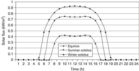
FIGURE 2.15 Daily variation of solar flux: horizontal E–W axis with N–S tracking.
The slope of this surface is given by:
![]() (2.27a)
(2.27a)
The surface orientation for this mode of tracking changes between 0° and 180°, if the solar azimuth angle passes through ±90°. For either hemisphere,
![]() (2.27b)
(2.27b)
Horizontal N–S axis with E–W tracking
For a plane rotated about a horizontal north–south axis with continuous adjustment to minimize the angle of incidence, θ can be obtained from (Kreith and Kreider, 1978; Duffie and Beckman, 1991),
![]() (2.28a)
(2.28a)
or from this equation (Meinel and Meinel, 1976):
![]() (2.28b)
(2.28b)
The basic geometry of this configuration is shown in Figure 2.10(d). The greatest advantage of this arrangement is that very small shadowing effects are encountered when more than one collector is used. These are present only at the first and last hours of the day. In this case the curve of the solar energy collected during the day is closer to a cosine curve function (see Figure 2.16).
FIGURE 2.16 Daily variation of solar flux: horizontal N–S axis and E–W tracking.
The slope of this surface is given by:
![]() (2.29a)
(2.29a)
The surface azimuth angle (Zs) is 90° or −90°, depending on the solar azimuth angle:
Comparison
The mode of tracking affects the amount of incident radiation falling on the collector surface in proportion to the cosine of the incidence angle. The amount of energy falling on a surface per unit area for the four modes of tracking for the summer and winter solstices and the equinoxes are shown in Table 2.2. This analysis has been performed with the same radiation model used to plot the solar flux figures in this section. Again, the type of the model used here is not important, because it is used for comparison purposes only. The performance of the various modes of tracking is compared with the full tracking, which collects the maximum amount of solar energy, shown as 100% in Table 2.2. From this table it is obvious that the polar and the N–S horizontal modes are the most suitable for one-axis tracking, since their performance is very close to the full tracking, provided that the low winter performance of the latter is not a problem.
Table 2.2
Comparison of Energy Received for Various Modes of Tracking
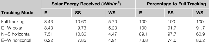
E = equinoxes, SS = summer solstice, WS = winter solstice.
Sun path diagrams
For practical purposes, instead of using the preceding equations, it is convenient to have the sun’s path plotted on a horizontal plane, called a sun path diagram, and to use the diagram to find the position of the sun in the sky at any time of the year. As can be seen from Eqs (2.12) and (2.13), the solar altitude angle, α, and the solar azimuth angle, z, are functions of latitude, L, hour angle, h, and declination, δ. In a two-dimensional plot, only two independent parameters can be used to correlate the other parameters; therefore, it is usual to plot different sun path diagrams for different latitudes. Such diagrams show the complete variations of hour angle and declination for a full year. Figure 2.17 shows the sun path diagram for 35°N latitude. Lines of constant declination are labeled by the value of the angles. Points of constant hour angles are clearly indicated. This figure is used in combination with Figure 2.7 or Eqs (2.5)–(2.7); that is, for a day in a year, Figure 2.7 or the equations can be used to estimate declination, which is then entered together with the time of day and converted to solar time using Eq. (2.3) in Figure 2.17 to estimate solar altitude and azimuth angles. It should be noted that Figure 2.17 applies for the Northern Hemisphere. For the Southern Hemisphere, the sign of the declination should be reversed. Figures A3.2 through A3.4 in Appendix 3 show the sun path diagrams for 30°, 40°, and 50°N latitudes.
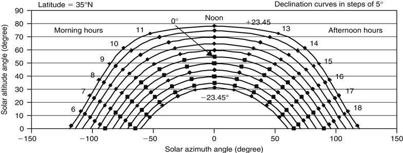
FIGURE 2.17 Sun path diagram for 35°N latitude.
Shadow determination
In the design of many solar energy systems, it is often required to estimate the possibility of the shading of solar collectors or the windows of a building by surrounding structures. To determine the shading, it is necessary to know the shadow cast as a function of time during every day of the year. Although mathematical models can be used for this purpose, a simpler graphical method is presented here, which is suitable for quick practical applications. This method is usually sufficient, since the objective is usually not to estimate exactly the amount of shading but to determine whether a position suggested for the placement of collectors is suitable or not.
Shadow determination is facilitated by the determination of a surface-oriented solar angle, called the solar profile angle. As shown in Figure 2.18, the solar profile angle, p, is the angle between the normal to a surface and the projection of the sun’s rays on a plane normal to the surface. In terms of the solar altitude angle, α, solar azimuth angle, z, and the surface azimuth angle, Zs, the solar profile angle p is given by the equation:
![]() (2.30a)
(2.30a)
A simplified equation is obtained when the surface faces due south, that is, Zs = 0°, given by:
![]() (2.30b)
(2.30b)
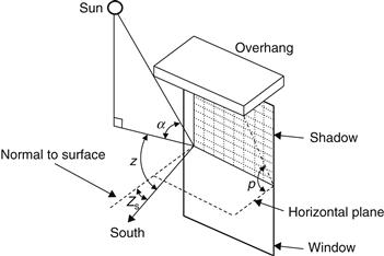
FIGURE 2.18 Geometry of solar profile angle, p, in a window overhang arrangement.
The sun path diagram is often very useful in determining the period of the year and hours of day when shading will take place at a particular location. This is illustrated in the following example.
EXAMPLE 2.8
A building is located at 35°N latitude and its side of interest is located 15° east of south. We want to investigate the time of the year that point x on the building will be shaded, as shown in Figure 2.19.
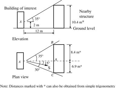
FIGURE 2.19 Shading of building in Example 2.8.
Solution
The upper limit of profile angle for shading point x is 35° and 15° west of true south. This is point A drawn on the sun path diagram, as shown in Figure 2.20. In this case, the solar profile angle is the solar altitude angle. Distance x–B is (8.42 + 122)1/2 = 14.6 m. For the point B, the altitude angle is tan(α) = 8.4/14.6 → α = 29.9°. Similarly, distance x–C is (6.92 + 122)1/2 = 13.8 m, and for point C, the altitude angle is tan(α) = 8.4/13.8 → α = 31.3°. Both points are as indicated on the sun path diagram in Figure 2.20.
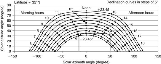
FIGURE 2.20 Sun path diagram for Example 2.8.
Therefore, point x on the wall of interest is shaded during the period indicated by the curve BAC in Figure 2.20. It is straightforward to determine the hours that shading occurs, whereas the time of year is determined by the declination.
Solar collectors are usually installed in multi-rows facing the true south. There is, hence, a need to estimate the possibility of shading by the front rows of the second and subsequent rows. The maximum shading, in this case, occurs at local solar noon, and this can easily be estimated by finding the noon altitude, αn, as given by Eq. (2.14) and checking whether the shadow formed shades on the second or subsequent collector rows. Generally, shading will not occur as long as the profile angle is greater than the angle θs, formed by the top corner of the front collector to the bottom end of the second row and the horizontal (see Figure 5.25). If the profile angle at any time is less than θs, then a portion of the collectors in the second and subsequent rows will be shaded from beam radiation.
EXAMPLE 2.9
Find the equation to estimate the shading caused by a fin on a window.
Solution
The fin and window assembly are shown in Figure 2.21.
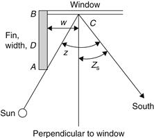
FIGURE 2.21 Fin and window assembly for Example 2.9.
From triangle ABC, the sides AB = D, BC = w, and angle A is z − Zs.
Therefore, distance w is estimated by w = D tan(z − Zs).
Shadow calculations for overhangs are examined in more detail in Chapter 6, Section 6.2.5.
2.3 Solar radiation
2.3.1 General
All substances, solid bodies as well as liquids and gases above the absolute zero temperature, emit energy in the form of electromagnetic waves.
The radiation that is important to solar energy applications is that emitted by the sun within the ultraviolet, visible, and infrared regions. Therefore, the radiation wavelength that is important to solar energy applications is between 0.15 and 3.0 μm. The wavelengths in the visible region lie between 0.38 and 0.72 μm.
This section initially examines issues related to thermal radiation, which includes basic concepts, radiation from real surfaces, and radiation exchanges between two surfaces. This is followed by the variation of extraterrestrial radiation, atmospheric attenuation, terrestrial irradiation, and total radiation received on sloped surfaces. Finally, it briefly describes radiation measuring equipment.
2.3.2 Thermal radiation
Thermal radiation is a form of energy emission and transmission that depends entirely on the temperature characteristics of the emissive surface. There is no intervening carrier, as in the other modes of heat transmission, that is, conduction and convection. Thermal radiation is in fact an electromagnetic wave that travels at the speed of light (C ≈ 300,000 km/s in a vacuum). This speed is related to the wavelength (λ) and frequency (ν) of the radiation as given by the equation:
![]() (2.31)
(2.31)
When a beam of thermal radiation is incident on the surface of a body, part of it is reflected away from the surface, part is absorbed by the body, and part is transmitted through the body. The various properties associated with this phenomenon are the fraction of radiation reflected, called reflectivity (ρ); the fraction of radiation absorbed, called absorptivity (α); and the fraction of radiation transmitted, called transmissivity (τ). The three quantities are related by the following equation:
![]() (2.32)
(2.32)
It should be noted that the radiation properties just defined are not only functions of the surface itself but also functions of the direction and wavelength of the incident radiation. Therefore, Eq. (2.32) is valid for the average properties over the entire wavelength spectrum. The following equation is used to express the dependence of these properties on the wavelength:
![]() (2.33)
(2.33)
The angular variation of absorptance for black paint is illustrated in Table 2.3 for incidence angles of 0–90°. The absorptance for diffuse radiation is approximately 0.90 (Löf and Tybout, 1972).
Table 2.3
Angular Variation of Absorptance for Black Paint
| Angle of Incidence (°) | Absorptance |
| 0–30 | 0.96 |
| 30–40 | 0.95 |
| 40–50 | 0.93 |
| 50–60 | 0.91 |
| 60–70 | 0.88 |
| 70–80 | 0.81 |
| 80–90 | 0.66 |
Reprinted from Löf and Tybout (1972) with permission from ASME.
Most solid bodies are opaque, so that τ = 0 and ρ + α = 1. If a body absorbs all the impinging thermal radiation such that τ = 0, ρ = 0, and α = 1, regardless of the spectral character or directional preference of the incident radiation, it is called a blackbody. This is a hypothetical idealization that does not exist in reality.
A blackbody is not only a perfect absorber but also characterized by an upper limit to the emission of thermal radiation. The energy emitted by a blackbody is a function of its temperature and is not evenly distributed over all wavelengths. The rate of energy emission per unit area at a particular wavelength is termed as the monochromatic emissive power. Max Planck was the first to derive a functional relation for the monochromatic emissive power of a blackbody in terms of temperature and wavelength. This was done by using the quantum theory, and the resulting equation, called Planck’s equation for blackbody radiation, is given
by:
![]() (2.34)
(2.34)
Ebλ = monochromatic emissive power of a blackbody (W/m2 μm).
T = absolute temperature of the surface (K).
C1 = constant = ![]() = 3.74177 × 10⁸ W μm4/m2.
= 3.74177 × 10⁸ W μm4/m2.
C2 = constant = hco/k = 1.43878 × 104 μm K.
h = Planck’s constant = 6.626069 × 10⁻³⁴ Js.
co = speed of light in vacuum = 2.9979 × 10⁸ m/s.
k = Boltzmann’s constant = 1.38065 × 10⁻²³ J/K.
Equation (2.34) is valid for a surface in a vacuum or a gas. For other mediums it needs to be modified by replacing C1 by C1/n2, where n is the index of refraction of the medium. By differentiating Eq. (2.34) and equating to 0, the wavelength corresponding to the maximum of the distribution can be obtained and is equal to λmaxT = 2897.8 μm K. This is known as Wien’s displacement law. Figure 2.22 shows the spectral radiation distribution for blackbody radiation at three temperature sources. The curves have been obtained by using the Planck’s equation.
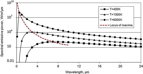
FIGURE 2.22 Spectral distribution of blackbody radiation.
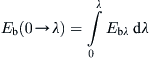
The total emissive power, Eb, and the monochromatic emissive power, Ebλ, of a blackbody are related by:
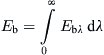 (2.35)
Substituting Eq. (2.34) into Eq. (2.35) and performing the integration results in the Stefan–Boltzmann law:
![]() (2.36a)
(2.36a)
where σ = the Stefan–Boltzmann constant = 5.6697 × 10⁻⁸ W/m2K4.
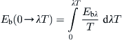
In many cases, it is necessary to know the amount of radiation emitted by a blackbody in a specific wavelength band λ1 → λ2. This is done by modifying Eq. (2.35) as:
 (2.36b)
Since the value of Ebλ depends on both λ and T, it is better to use both variables as:
 (2.36c)
Therefore, for the wavelength band of λ1 → λ2, we get:
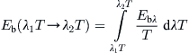 (2.36d)
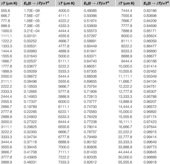
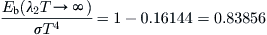
which results in Eb(0 → λ1T) − Eb(0 → λ2T). Table 2.4 presents a tabulation of Eb(0 → λT) as a fraction of the total emissive power, Eb = σT4, for various values of λT, also called fraction of radiation emitted from a blackbody at temperature T in the wavelength band from λ = 0 to λ, f0-λT or for a particular temperature, fλ. The values are not rounded, because the original table, suggested by Dunkle (1954), recorded λT in micrometer-degrees Rankine (μm °R), which were converted to micrometer-Kelvins (μm K) in Table 2.4.
Table 2.4
Fraction of Blackbody Radiation as a Function of λT
The fraction of radiation emitted from a blackbody at temperature T in the wavelength band from λ = 0 to λ can be solved easily on a computer using the polynomial form, with about 10 summation terms for good accuracy, suggested by Siegel and Howell (2002):
![]() (2.36e)
(2.36e)
A blackbody is also a perfect diffuse emitter, so its intensity of radiation, Ib, is a constant in all directions, given by:
![]() (2.37)
(2.37)
Of course, real surfaces emit less energy than corresponding blackbodies. The ratio of the total emissive power, E, of a real surface to the total emissive power, Eb, of a blackbody, both at the same temperature, is called the emissivity (ε) of a real surface; that is,
![]() (2.38)
(2.38)
The emissivity of a surface not only is a function of surface temperature but also depends on wavelength and direction. In fact, the emissivity given by Eq. (2.38) is the average value over the entire wavelength range in all directions, and it is often referred to as the total or hemispherical emissivity. Similar to Eq. (2.38), to express the dependence on wavelength, the monochromatic or spectral emissivity, ελ, is defined as the ratio of the monochromatic emissive power, Eλ, of a real surface to the monochromatic emissive power, Ebλ, of a blackbody, both at the same wavelength and temperature:
![]() (2.39)
(2.39)
Kirchoff’s law of radiation states that, for any surface in thermal equilibrium, monochromatic emissivity is equal to monochromatic absorptivity:
![]() (2.40)
(2.40)
The temperature (T) is used in Eq. (2.40) to emphasize that this equation applies only when the temperatures of the source of the incident radiation and the body itself are the same. It should be noted, therefore, that the emissivity of a body on earth (at normal temperature) cannot be equal to solar radiation (emitted from the sun at T = 5760 K). Equation (2.40) can be generalized as:
![]() (2.41)
(2.41)
Equation (2.41) relates the total emissivity and absorptivity over the entire wavelength. This generalization, however, is strictly valid only if the incident and emitted radiation have, in addition to the temperature equilibrium at the surfaces, the same spectral distribution. Such conditions are rarely met in real life; to simplify the analysis of radiation problems, however, the assumption that monochromatic properties are constant over all wavelengths is often made. Such a body with these characteristics is called a gray body.
Similar to Eq. (2.37) for a real surface, the radiant energy leaving the surface includes its original emission and any reflected rays. The rate of total radiant energy leaving a surface per unit surface area is called the radiosity (J), given by:
![]() (2.42)
(2.42)
Eb = blackbody emissive power per unit surface area (W/m2).
H = irradiation incident on the surface per unit surface area (W/m2).
ε = emissivity of the surface.
ρ = reflectivity of the surface.
There are two idealized limiting cases of radiation reflection: the reflection is called specular if the reflected ray leaves at an angle with the normal to the surface equal to the angle made by the incident ray, and it is called diffuse if the incident ray is reflected uniformly in all directions. Real surfaces are neither perfectly specular nor perfectly diffuse. Rough industrial surfaces, however, are often considered as diffuse reflectors in engineering calculations.
A real surface is both a diffuse emitter and a diffuse reflector and hence, it has diffuse radiosity; that is, the intensity of radiation from this surface (I) is constant in all directions. Therefore, the following equation is used for a real surface:
EXAMPLE 2.10
A glass with transmissivity of 0.92 is used in a certain application for wavelengths 0.3 and 3.0 μm. The glass is opaque to all other wavelengths. Assuming that the sun is a blackbody at 5760 K and neglecting atmospheric attenuation, determine the percent of incident solar energy transmitted through the glass. If the interior of the application is assumed to be a blackbody at 373 K, determine the percent of radiation emitted from the interior and transmitted out through the glass.
Solution
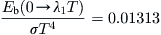
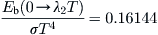
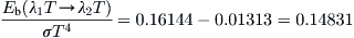
For the incoming solar radiation at 5760 K, we have:


From Table 2.4 by interpolation, we get:
Therefore, the percent of solar radiation incident on the glass in the wavelength range 0.3–3 μm is:
In addition, the percentage of radiation transmitted through the glass is 0.92 × 94.61 = 87.04%.
For the outgoing infrared radiation at 373 K, we have:


From Table 2.4, we get:
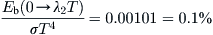
The percent of outgoing infrared radiation incident on the glass in the wavelength 0.3–3 μm is 0.1%, and the percent of this radiation transmitted out through the glass is only 0.92 × 0.1 = 0.092%. This example, in fact, demonstrates the principle of the greenhouse effect; that is, once the solar energy is absorbed by the interior objects, it is effectively trapped.
EXAMPLE 2.11
A surface has a spectral emissivity of 0.87 at wavelengths less than 1.5 μm, 0.65 at wavelengths between 1.5 and 2.5 μm, and 0.4 at wavelengths longer than 2.5 μm. If the surface is at 1000 K, determine the average emissivity over the entire wavelength and the total emissive power of the surface.
Solution
From the data given, we have:


From Table 2.4 by interpolation, we get:
and
Therefore,
and
The average emissive power over the entire wavelength is given by:

and the total emissive power of the surface is:

The other properties of the materials can be obtained using the Kirchhoff’s law given by Eq. (2.40) or Eq. (2.41) as demonstrated by the following example.
EXAMPLE 2.12
The variation of the spectral absorptivity of an opaque surface is 0.2 up to the wavelength of 2 μm and 0.7 for bigger wavelengths. Estimate the average absorptivity and reflectivity of the surface from radiation emitted from a source at 2500 K. Determine also the average emissivity of the surface at 3000 K.
Solution
At a temperature of 2500 K:

Therefore, from Table 2.4: ![]()
The average absorptivity of the surface is:

As the surface is opaque from Eq. (2.32): α + ρ = 1. So, ρ = 1 − α = 1 − 0.383 = 0.617.
Using Kirchhoff’s law, from Eq. (2.41) ε(T) = α(T). So the average emissivity of this surface at T = 3000 K is:

Therefore, from Table 2.4: ![]()
And ε(T) = ε1fλ1 + ε2(1 − fλ1) = (0.2)(0.73777) + (0.7)(1 – 0.73777) = 0.331.
2.3.3 Transparent plates
When a beam of radiation strikes the surface of a transparent plate at angle θ1, called the incidence angle, as shown in Figure 2.23, part of the incident radiation is reflected and the remainder is refracted, or bent, to angle θ2, called the refraction angle, as it passes through the interface. Angle θ1 is also equal to the angle at which the beam is specularly reflected from the surface. Angles θ1 and θ2 are not equal when the density of the plane is different from that of the medium through which the radiation travels. Additionally, refraction causes the transmitted beam to be bent toward the perpendicular to the surface of higher density. The two angles are related by the Snell’s law:
![]() (2.44)
(2.44)
where n1 and n2 are the refraction indices and n is the ratio of refraction index for the two media forming the interface. The refraction index is the determining factor for the reflection losses at the interface. A typical value of the refraction index is 1.000 for air, 1.526 for glass, and 1.33 for water.
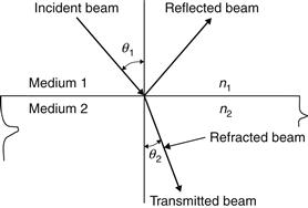
FIGURE 2.23 Incident and refraction angles for a beam passing from a medium with refraction index n1 to a medium with refraction index n2.
Expressions for perpendicular and parallel components of radiation for smooth surfaces were derived by Fresnel as:
![]() (2.45)
(2.45)
![]() (2.46)
(2.46)
Equation (2.45) represents the perpendicular component of unpolarized radiation and Eq. (2.46) represents the parallel one. It should be noted that parallel and perpendicular refer to the plane defined by the incident beam and the surface normal.
Properties are evaluated by calculating the average of these two components as:
![]() (2.47)
(2.47)
For normal incidence, both angles are 0 and Eq. (2.47) can be combined with Eq. (2.44) to yield:
![]() (2.48)
(2.48)
If one medium is air (n = 1.0), then Eq. (2.48) becomes:
![]() (2.49)
(2.49)
Similarly, the transmittance, τr (subscript r indicates that only reflection losses are considered), can be calculated from the average transmittance of the two components as follows:
![]() (2.50a)
(2.50a)
For a glazing system of N covers of the same material, it can be proven that:
![]() (2.50b)
(2.50b)
The transmittance, τα (subscript α indicates that only absorption losses are considered), can be calculated from:
![]() (2.51)
(2.51)
where K is the extinction coefficient, which can vary from 4m−1 (for high-quality glass) to 32m−1 (for low-quality glass), and L is the thickness of the glass cover.
The transmittance, reflectance, and absorptance of a single cover (by considering both reflection and absorption losses) are given by the following expressions. These expressions are for the perpendicular components of polarization, although the same relations can be used for the parallel components:
![]() (2.52a)
(2.52a)
![]() (2.52b)
(2.52b)
![]() (2.52c)
(2.52c)
Since, for practical collector covers, τα is seldom less than 0.9 and r is of the order of 0.1, the transmittance of a single cover becomes:
![]() (2.53)
(2.53)
The absorptance of a cover can be approximated by neglecting the last term of Eq. (2.52c):
![]() (2.54)
(2.54)
and the reflectance of a single cover could be found (keeping in mind that ρ = 1 − α − τ) as:
![]() (2.55)
(2.55)
For a two-cover system of not necessarily same materials, the following equation can be obtained (subscript 1 refers to the outer cover and 2 to the inner one):
![]() (2.56)
(2.56)
![]() (2.57)
(2.57)
EXAMPLE 2.13
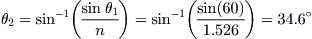
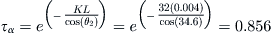
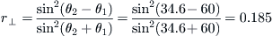
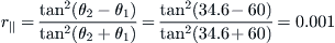
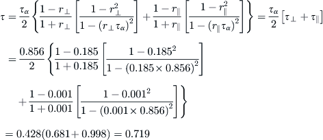
A solar energy collector uses a single glass cover with a thickness of 4 mm. In the visible solar range, the refraction index of glass, n, is 1.526 and its extinction coefficient K is 32m−1. Calculate the reflectivity, transmissivity, and absorptivity of the glass sheet for the angle of incidence of 60° and at normal incidence (0°).
Solution
Angle of incidence = 60°
From Eq. (2.44), the refraction angle θ2 is calculated as:
From Eq. (2.51), the transmittance can be obtained as:
From Eqs (2.45) and (2.46),
From Eqs (2.52a)–(2.52c), we have:


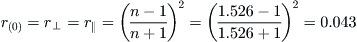
Normal incidence
At normal incidence, θ1 = 0° and θ2 = 0°. In this case, τα is equal to 0.880. There is no polarization at normal incidence; therefore, from Eq. (2.49),
From Eqs (2.52a)–(2.52c), we have:


Radiation exchange between surfaces
When studying the radiant energy exchanged between two surfaces separated by a non-absorbing medium, one should consider not only the temperature of the surfaces and their characteristics but also their geometric orientation with respect to each other. The effects of the geometry of radiant energy exchange can be analyzed conveniently by defining the term view factor, F12, to be the fraction of radiation leaving surface A1 that reaches surface A2. If both surfaces are black, the radiation leaving surface A1 and arriving at surface A2 is Eb1A1F12, and the radiation leaving surface A2 and arriving at surface A1 is Eb2A2F21. If both surfaces are black and absorb all incident radiation, the net radiation exchange is given by:
![]() (2.58)
(2.58)
If both surfaces are of the same temperature, Eb1 = Eb2 and Q12 = 0. Therefore,
![]() (2.59)
(2.59)
It should be noted that Eq. (2.59) is strictly geometric in nature and valid for all diffuse emitters, irrespective of their temperatures. Therefore, the net radiation exchange between two black surfaces is given by:
![]() (2.60)
(2.60)
From Eq. (2.36a), Eb = σT4, Eq. (2.60) can be written as:
![]() (2.61)
(2.61)
where T1 and T2 are the temperatures of surfaces A1 and A2, respectively. As the term (Eb1 − Eb2) in Eq. (2.60) is the energy potential difference that causes the transfer of heat, in a network of electric circuit analogy, the term 1/A1F12 = 1/A2F21 represents the resistance due to the geometric configuration of the two surfaces.
When surfaces other than black are involved in radiation exchange, the situation is much more complex, because multiple reflections from each surface must be taken into consideration. For the simple case of opaque gray surfaces, for which ε = α, the reflectivity ρ = 1 − α = 1 − ε. From Eq. (2.42), the radiosity of each surface is given by:
![]() (2.62)
(2.62)
The net radiant energy leaving the surface is the difference between the radiosity, J, leaving the surface and the irradiation, H, incident on the surface; that is,
![]() (2.63)
(2.63)
Combining Eqs (2.62) and (2.63) and eliminating irradiation H results in:
![]() (2.64)
(2.64)
Therefore, the net radiant energy leaving a gray surface can be regarded as the current in an equivalent electrical network when a potential difference (Eb − J) is overcome across a resistance R = (1 − ε)/Aε. This resistance, called surface resistance, is due to the imperfection of the surface as an emitter and absorber of radiation as compared with a black surface.
By considering the radiant energy exchange between two gray surfaces, A1 and A2, the radiation leaving surface A1 and arriving at surface A2 is J1A1F12, where J is the radiosity, given by Eq. (2.42). Similarly, the radiation leaving surface A2 and arriving surface A1 is J2A2F21. The net radiation exchange between the two surfaces is given by:
![]() (2.65)
(2.65)
Therefore, due to the geometric orientation that applies between the two potentials, J1 and J2, when two gray surfaces exchange radiant energy, there is a resistance, called space resistance, R = 1/A1F12 = 1/A2F21.
An equivalent electric network for two the gray surfaces is illustrated in Figure 2.24. By combining the surface resistance, (1 − ε)/Aε for each surface and the space (or geometric) resistance, 1/A1F12 = 1/A2F21, between the surfaces, as shown in Figure 2.24, the net rate of radiation exchange between the two surfaces is equal to the overall potential difference divided by the sum of resistances, given by:
 (2.66)
In solar energy applications, the following geometric orientations between two surfaces are of particular interest.
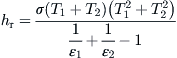
A. For two infinite parallel surfaces, A1 = A2 = A and F12 = 1, Eq. (2.66) becomes:
![]() (2.67)
(2.67)
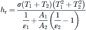
B. For two concentric cylinders, F12 = 1 and Eq. (2.66) becomes:
![]() (2.68)
(2.68)
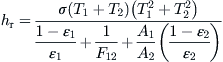
C. For a small convex surface, A1, completely enclosed by a very large concave surface, A2, A1 << A2 and F12 = 1, then Eq. (2.66) becomes:
![]() (2.69)
(2.69)
The last equation also applies for a flat-plate collector cover radiating to the surroundings, whereas case B applies in the analysis of a parabolic trough collector receiver where the receiver pipe is enclosed in a glass cylinder.
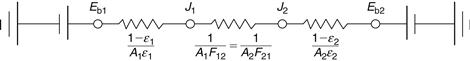
FIGURE 2.24 Equivalent electrical network for radiation exchange between two gray surfaces.
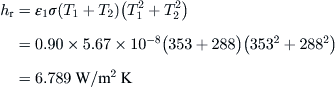
As can be seen from Eqs (2.67)–(2.69), the rate of radiative heat transfer between surfaces depends on the difference of the fourth power of the surface temperatures. In many engineering calculations, however, the heat transfer equations are linearized in terms of the differences of temperatures to the first power. For this purpose, the following mathematical identity is used:
![]() (2.70)
(2.70)
Therefore, Eq. (2.66) can be written as:
![]() (2.71)
(2.71)
with the radiation heat transfer coefficient, hr, defined as:
 (2.72)
For the special cases mentioned previously, the expressions for hr are as follows:
 (2.73)
 (2.74)
![]() (2.75)
(2.75)
It should be noted that the use of these linearized radiation equations in terms of hr is very convenient when the equivalent network method is used to analyze problems involving conduction and/or convection in addition to radiation. The radiation heat transfer coefficient, hr, is treated similarly to the convection heat transfer coefficient, hc, in an electric equivalent circuit. In such a case, a combined heat transfer coefficient can be used, given by:
![]() (2.76)
(2.76)
In this equation, it is assumed that the linear temperature difference between the ambient fluid and the walls of the enclosure and the surface and the enclosure substances are at the same temperature.
EXAMPLE 2.14
The glass of a 1 × 2 m flat-plate solar collector is at a temperature of 80 °C and has an emissivity of 0.90. The environment is at a temperature of 15 °C. Calculate the convection and radiation heat losses if the convection heat transfer coefficient is 5.1 W/m2K.
Solution
In the following analysis, the glass cover is denoted by subscript 1 and the environment by 2. The radiation heat transfer coefficient is given by Eq. (2.75):
Therefore, from Eq. (2.76),

Finally,

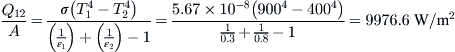
EXAMPLE 2.15
Two very large parallel plates are maintained at uniform temperatures of 900 K and 400 K. The emissivities of the two surfaces are 0.3 and 0.8, respectively. What is the radiation heat transfer between the two surfaces?
Solution
As the areas of the two surfaces are not given the estimation is given per unit surface area of the plates. As the two plates are very large and parallel, Eq. (2.67) apply, so:
EXAMPLE 2.16
Two very long concentric cylinders of diameters 30 and 50 cm are maintained at uniform temperatures of 850 K and 450 K. The emissivities of the two surfaces are 0.9 and 0.6, respectively. The space between the two cylinders is evacuated. What is the radiation heat transfer between the two cylinders per unit length of the cylinders?
Solution
For concentric cylinders Eq. (2.68) applies. Therefore,

2.3.5 Extraterrestrial solar radiation
The amount of solar energy per unit time, at the mean distance of the earth from the sun, received on a unit area of a surface normal to the sun (perpendicular to the direction of propagation of the radiation) outside the atmosphere is called the solar constant, Gsc. This quantity is difficult to measure from the surface of the earth because of the effect of the atmosphere. A method for the determination of the solar constant was first given in 1881 by Langley (Garg, 1982), who had given his name to the units of measurement as Langleys per minute (calories per square centimeter per minute). This was changed by the SI system to Watts per square meter (W/m2).
When the sun is closest to the earth, on January 3, the solar heat on the outer edge of the earth’s atmosphere is about 1400 W/m2; and when the sun is farthest away, on July 4, it is about 1330 W/m2.
Throughout the year, the extraterrestrial radiation measured on the plane normal to the radiation on the Nth day of the year, Gon, varies between these limits, as indicated in Figure 2.25, in the range of 3.3% and can be calculated by (Duffie and Beckman, 1991; Hsieh, 1986):
![]() (2.77)
(2.77)
Gon = extraterrestrial radiation measured on the plane normal to the radiation on the Nth day of the year (W/m2).
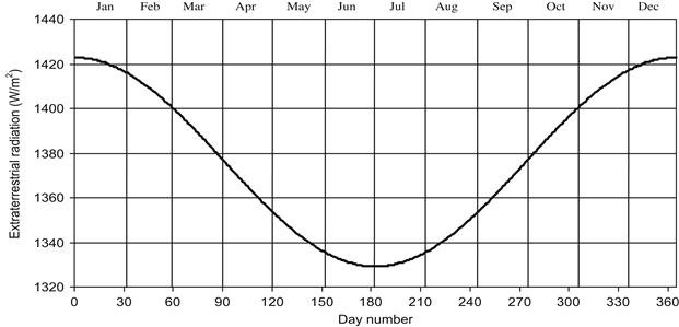
FIGURE 2.25 Variation of extraterrestrial solar radiation with the time of year.
The latest value of Gsc is 1366.1 W/m2. This was adopted in 2000 by the American Society for Testing and Materials (ASTM), which developed an AM0 reference spectrum (ASTM E-490). The ASTM E-490 Air Mass Zero solar spectral irradiance is based on data from satellites, space shuttle missions, high-altitude aircraft, rocket soundings, ground-based solar telescopes, and modeled spectral irradiance. The spectral distribution of extraterrestrial solar radiation at the mean sun–earth distance is shown in Figure 2.26. The spectrum curve of Figure 2.26 is based on a set of data included in ASTM E-490 (Solar Spectra, 2007).
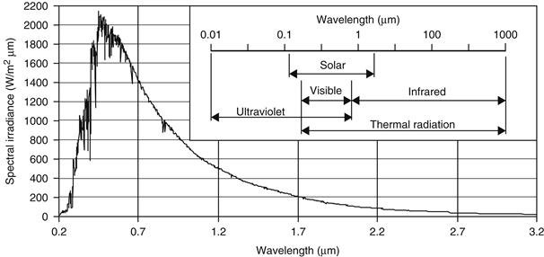
FIGURE 2.26 Standard curve giving a solar constant of 1366.1 W/m2 and its position in the electromagnetic radiation spectrum.
When a surface is placed parallel to the ground, the rate of solar radiation, GoH, incident on this extraterrestrial horizontal surface at a given time of the year is given by:
![]() (2.78)
(2.78)
The total radiation, Ho, incident on an extraterrestrial horizontal surface during a day can be obtained by the integration of Eq. (2.78) over a period from sunrise to sunset. The resulting equation is:
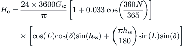 (2.79)
where hss is the sunset hour in degrees, obtained from Eq. (2.15). The units of Eq. (2.79) are joules per square meter (J/m2).
To calculate the extraterrestrial radiation on a horizontal surface for an hour period, Eq. (2.78) is integrated between hour angles, h1 and h2 (h2 is larger). Therefore,
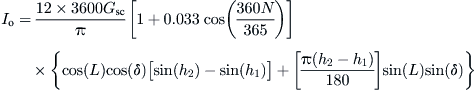 (2.80)
It should be noted that the limits h1 and h2 may define a time period other than 1 h.
EXAMPLE 2.17
Determine the extraterrestrial normal radiation and the extraterrestrial radiation on a horizontal surface on March 10 at 2:00 pm solar time for 35°N latitude. Determine also the total solar radiation on the extraterrestrial horizontal surface for the day.
Solution
The declination on March 10 (N = 69) is calculated from Eq. (2.5):
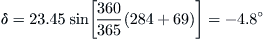
The hour angle at 2:00 pm solar time is calculated from Eq. (2.8):

The hour angle at sunset is calculated from Eq. (2.15):

The extraterrestrial normal radiation is calculated from Eq. (2.77):

The extraterrestrial radiation on a horizontal surface is calculated from Eq. (2.78):

The total radiation on the extraterrestrial horizontal surface is calculated from Eq. (2.79):

A list of definitions that includes those related to solar radiation is found in Appendix 2. The reader should familiarize himself or herself with the various terms and specifically with irradiance, which is the rate of radiant energy falling on a surface per unit area of the surface (units, watts per square meter [W/m2] symbol, G), whereas irradiation is incident energy per unit area on a surface (units, joules per square meter [J/m2]), obtained by integrating irradiance over a specified time interval. Specifically, for solar irradiance this is called insolation. The symbols used in this book are H for insolation for a day and I for insolation for an hour. The appropriate subscripts used for G, H, and I are beam (B), diffuse (D), and ground-reflected (G) radiation.
Atmospheric attenuation
The solar heat reaching the earth’s surface is reduced below Gon because a large part of it is scattered, reflected back out into space, and absorbed by the atmosphere. As a result of the atmospheric interaction with the solar radiation, a portion of the originally collimated rays becomes scattered or non-directional. Some of this scattered radiation reaches the earth’s surface from the entire sky vault. This is called the diffuse radiation. The solar heat that comes directly through the atmosphere is termed direct or beam radiation. The insolation received by a surface on earth is the sum of diffuse radiation and the normal component of beam radiation. The solar heat at any point on earth depends on:
2. The distance traveled through the atmosphere to reach that point
3. The amount of haze in the air (dust particles, water vapor, etc.)
4. The extent of the cloud cover
The earth is surrounded by atmosphere that contains various gaseous constituents, suspended dust, and other minute solid and liquid particulate matter and clouds of various types. As the solar radiation travels through the earth’s atmosphere, waves of very short length, such as X-rays and gamma rays, are absorbed in the ionosphere at extremely high altitude. The waves of relatively longer length, mostly in the ultraviolet range, are then absorbed by the layer of ozone (O3), located about 15–40 km above the earth’s surface. In the lower atmosphere, bands of solar radiation in the infrared range are absorbed by water vapor and carbon dioxide. In the long-wavelength region, since the extraterrestrial radiation is low and the H2O and CO2 absorption is strong, little solar energy reaches the ground.
Therefore, the solar radiation is depleted during its passage though the atmosphere before reaching the earth’s surface. The reduction of intensity with increasing zenith angle of the sun is generally assumed to be directly proportional to the increase in air mass, an assumption that considers the atmosphere to be unstratified with regard to absorbing or scattering impurities.
The degree of attenuation of solar radiation traveling through the earth’s atmosphere depends on the length of the path and the characteristics of the medium traversed. In solar radiation calculations, one standard air mass is defined as the length of the path traversed in reaching the sea level when the sun is at its zenith (the vertical at the point of observation). The air mass is related to the zenith angle, Φ (Figure 2.27), without considering the earth’s curvature, by the equation:
![]() (2.81)
(2.81)
Therefore, at sea level when the sun is directly overhead, that is, when Φ = 0°, m = 1 (air mass one); and when Φ = 60°, we get m = 2 (air mass two). Similarly, the solar radiation outside the earth’s atmosphere is at air mass zero. The graph of direct normal irradiance (solar spectrum) at ground level for air mass 1.5 is shown in Appendix 4.
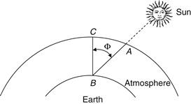
FIGURE 2.27 Air mass definition.
Terrestrial irradiation
A solar system frequently needs to be judged on its long-term performance. Therefore, knowledge of long-term monthly average daily insolation data for the locality under consideration is required. Daily mean total solar radiation (beam plus diffuse) incident on a horizontal surface for each month of the year is available from various sources, such as radiation maps or a country’s meteorological service (see Section 2.4). In these sources, data, such as 24 h average temperature, monthly average daily radiation on a horizontal surface ![]() (MJ/m2 day), and monthly average clearness index,
(MJ/m2 day), and monthly average clearness index, ![]() , are given together with other parameters, which are not of interest here.2 The monthly average clearness index,
, are given together with other parameters, which are not of interest here.2 The monthly average clearness index, ![]() , is defined as:
, is defined as:
![]() (2.82a)
(2.82a)
![]() = monthly average daily total radiation on a terrestrial horizontal surface (MJ/m2 day).
= monthly average daily total radiation on a terrestrial horizontal surface (MJ/m2 day).
![]() = monthly average daily total radiation on an extraterrestrial horizontal surface (MJ/m2 day).
= monthly average daily total radiation on an extraterrestrial horizontal surface (MJ/m2 day).
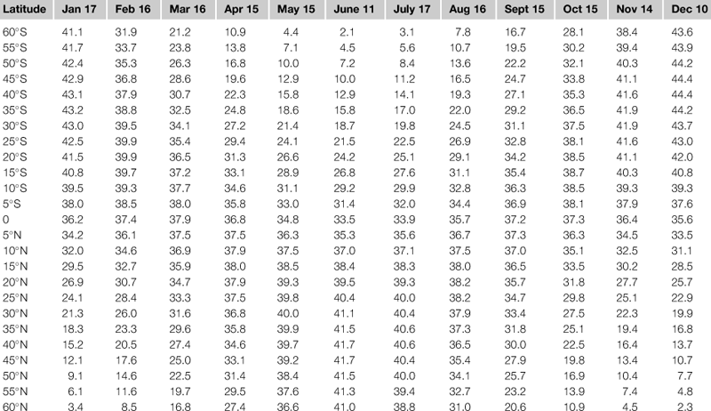
The bar over the symbols signifies a long-term average. The value of ![]() can be calculated from Eq. (2.79) by choosing a particular day of the year in the given month for which the daily total extraterrestrial insolation is estimated to be the same as the monthly mean value. Table 2.5 gives the values of
can be calculated from Eq. (2.79) by choosing a particular day of the year in the given month for which the daily total extraterrestrial insolation is estimated to be the same as the monthly mean value. Table 2.5 gives the values of ![]() for each month as a function of latitude, together with the recommended dates of each month that would give the mean daily values of
for each month as a function of latitude, together with the recommended dates of each month that would give the mean daily values of ![]() . The day number and the declination of the day for the recommended dates are shown in Table 2.1. For the same days, the monthly average daily extraterrestrial insolation on a horizontal surface for various months in kilowatt hours per square meter (kWh/m2 day) for latitudes −60° to +60° is also shown graphically in Figure A3.5 in Appendix 3, from which we can easily interpolate.
. The day number and the declination of the day for the recommended dates are shown in Table 2.1. For the same days, the monthly average daily extraterrestrial insolation on a horizontal surface for various months in kilowatt hours per square meter (kWh/m2 day) for latitudes −60° to +60° is also shown graphically in Figure A3.5 in Appendix 3, from which we can easily interpolate.
Table 2.5
Monthly Average Daily Extraterrestrial Insolation on Horizontal Surface (MJ/m2)
Further to Eq. (2.82a) the daily clearness index KT, can be defined as the ratio of the radiation for a particular day to the extraterrestrial radiation for that day given by:
![]() (2.82b)
(2.82b)
Similarly, an hourly clearness index kT, can be defined given by:
![]() (2.82c)
(2.82c)
In all these equations the values of ![]() , H, and I can be obtained from measurements of total solar radiation on horizontal using a pyranometer (see section 2.3.9).
, H, and I can be obtained from measurements of total solar radiation on horizontal using a pyranometer (see section 2.3.9).
To predict the performance of a solar system, hourly values of radiation are required. Because in most cases these types of data are not available, long-term average daily radiation data can be utilized to estimate long-term average radiation distribution. For this purpose, empirical correlations are usually used. Two such frequently used correlations are the Liu and Jordan (1977) correlation for the diffuse radiation and the Collares-Pereira and Rabl (1979) correlation for the total radiation.
According to the Liu and Jordan (1977) correlation,
![]() (2.83)
(2.83)
rd = ratio of hourly diffuse radiation to daily diffuse radiation (=ID/HD).
hss = sunset hour angle (degrees).
h = hour angle in degrees at the midpoint of each hour.
According to the Collares-Pereira and Rabl (1979) correlation,
![]() (2.84a)
(2.84a)
r = ratio of hourly total radiation to daily total radiation (=I/H).
![]() (2.84b)
(2.84b)
![]() (2.84c)
(2.84c)
EXAMPLE 2.18
Given the following empirical equation,
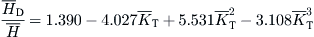
where ![]() is the monthly average daily diffuse radiation on horizontal surface—see Eq. (2.105a)—estimate the average total radiation and the average diffuse radiation between 11:00 am and 12:00 pm solar time in the month of July on a horizontal surface located at 35°N latitude. The monthly average daily total radiation on a horizontal surface,
is the monthly average daily diffuse radiation on horizontal surface—see Eq. (2.105a)—estimate the average total radiation and the average diffuse radiation between 11:00 am and 12:00 pm solar time in the month of July on a horizontal surface located at 35°N latitude. The monthly average daily total radiation on a horizontal surface, ![]() , in July at the surface location is 23.14 MJ/m2 day.
, in July at the surface location is 23.14 MJ/m2 day.
Solution
From Table 2.5 at 35° N latitude for July, ![]() . Therefore,
. Therefore,
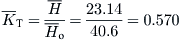
Therefore,

and

From Table 2.5, the recommended average day for the month is July 17 (N = 198). The solar declination is calculated from Eq. (2.5) as:

The sunset hour angle is calculated from Eq. (2.15) as:

The middle point of the hour from 11:00 am to 12:00 pm is 0.5 h from solar noon, or hour angle is −7.5°. Therefore, from Eqs. (2.84b), (2.84c) and (2.84a), we have:


From Eq. (2.83), we have:

Finally,


Leave a Reply