
With the procedure described earlier in this chapter for the performance evaluation of solar energy collectors, the collector performance equation is derived which can be used for the prediction of its output under any conditions. The basic aim of the collector testing is the determination of the collector thermal efficiency under specific conditions and as can be seen the behavior of the collector can be obtained with either a 2- or a 3-parameter single-node steady-state model given by Eqs (4.4) and (4.11), respectively, for an FPC or from the quasi-dynamic state model or dynamic test method given by Eq. (4.34).
During the experimental phase, the inlet and outlet temperatures are measured, as well as the solar energy and the basic climatic quantities, whereas in analyzing the data a least-squares fit is performed on the measured data to determine the various parameters of the above equations. All these measurements and calculations have certain uncertainties which need to be considered according to Annex K of EN 12975-2:2006. As mentioned in the standard the aim of the annex is to provide a general guidance for the assessment of uncertainty in the result of solar collector testing performed according to the standard. Uncertainty values are expressed in the same way as standard deviations.
It should be noted that the proposed methodology is one of the possible approaches for the assessment of uncertainty. The particular approach to be followed by a testing laboratory is often recommended by the accreditation body responsible for certifying the laboratory. The present approach is given here, however, as it is included in the above-mentioned standard.
Specifically, it is assumed that the behavior of the collector can be described by an M-parameter single-node steady-state or quasi-dynamic model given by:
![]() (4.39)
(4.39)
p1, p2, …, pM are quantities, the values of which are determined experimentally through testing
c1, c2, …, cM are characteristic constants of the collector that are determined through testing.
In the case of the steady-state model given by Eq. (4.11), M = 3, c1 = η0, c2 = U1, c3 = U2, p1 = 1, p2 = (Ti − Ta)/Gt and p3 = (Ti − Ta)2/Gt. During the experimental phase, the various quantities mentioned above are measured in J steady-state or quasi-dynamic state points, depending on the model used. From these primary measurements the values of parameters η, p1, p2, …, pM are derived for each point of observation j, j = 1, …, J. Generally, the experimental procedure of the testing leads to a formation of a group of J observations which comprise, for each one of the J testing points, the values of ηj, p1, j, p2, j, …, pM, j.
For the determination of uncertainties, it is required to calculate the respective combined standard uncertainties u(ηj), u(p1, j), …, u(pM, j) in each observations point. Additionally in practice, these uncertainties are almost never constant and the same for all points, but that each testing point has its own standard deviation which needs to be estimated.
According to the Standard and Mathioulakis et al. (1999), generally standard uncertainties in experimental data are of two types: Type A and Type B; the former are the uncertainties determined by statistical means while the latter are determined by other means.
The objective of a measurement is to determine the value of the measurand, that is, the value of the particular quantity to be measured. A measurement therefore begins with an appropriate specification of the measurand, the method of measurement, and the measurement procedure. It is now widely recognized that, when all of the known or suspected components of error have been evaluated and the appropriate corrections have been applied, there still remains an uncertainty about the correctness of the stated result, that is, a doubt about how well the result of the measurement represents the value of the quantity being measured (BIPM et al., 2008). The uncertainty of measurement is defined as the parameter associated with the result of a measurement characterizing the dispersion of the values that could reasonably be attributed to the measurand (Sabatelli et al., 2002).
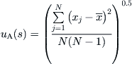
Type A uncertainties uA(s) derive from the statistical analysis of repeated measurements at each point of the steady-state or quasi-dynamic state operation of the collector. When a measurement is repeated under repeatability conditions, one can observe a scatter of the measured values. Variations in repeated observations are assumed to arise because influence quantities that can affect the measurement result are not held completely constant. Therefore, for the steady-state test, Type A uncertainty is the standard deviation of the mean of N measurements taken for each quantity measured during testing given by:
 (4.40)
As is evident from Eq. (4.40), Type A uncertainty depends upon the specific conditions of the measurement and thus can be reduced by increasing the number of measurements (Sabatelli et al., 2002). In the case of the quasi-dynamic test, where no arithmetic mean of the repetitive measurements is used, uncertainty uA(s) can be equal to zero.
By nature, Type A uncertainties depend on the specific conditions of the test and they include the fluctuations of the measured quantities during the measurement which lie within the limits implied by the Standard and the fluctuations of the testing conditions such as the air speed and the global diffuse irradiance.
Type B uncertainties derive from a combination of uncertainties over the whole measurement, taking into account all available data such as sensor uncertainty, data logger uncertainty, and uncertainty resulting from the possible differences between the measured values perceived by the measuring device (Mathioulakis et al., 1999). Therefore, Type B uncertainties, being dependent upon the measuring instrument, cannot be reduced by augmenting the number of measurements. Relevant information should be obtained from calibration certificates or other technical specifications of the instruments used. The uncertainty u(s) associated with a measurement s is the result of a combination of the Type B uncertainty uB(s), which is a characteristic feature of the calibration setup, and of the Type A uncertainty uA(s), which represents fluctuation during the sampling of data.
In some cases, it may be possible to estimate only bounds (upper and lower limits) for the value of a quantity X, in particular, to state that “the probability that the value of X lies within the interval a− to a+ for all practical purposes is equal to one and the probability that X lies outside this interval is essentially zero”. If there is no specific knowledge about the possible values of i within the interval, one can only assume that it is equally probable for X to lie anywhere within it. Then x, the expectation or expected value of X, is the midpoint of the interval, x = (a− + a+)/2, with associated standard uncertainty (BIPM et al., 2008):
![]() (4.41)
(4.41)
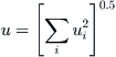
If there is more than one independent source of uncertainty (Type A or Type B) uk, the final uncertainty is calculated according to the general law of uncertainties combination:
 (4.42)
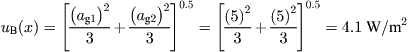
For example instruments that have two uncertainties, as, for example, the pyranometer that usually has a non-linearity error, of say ±5 W/m2, and temperature dependence, of say ±5 W/m2 within the actual operating range, by applying the law of propagation of errors, the respective standard uncertainty is given by:
 (4.43)
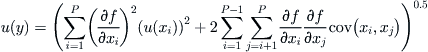
The term combined standard uncertainty means the standard uncertainty in a result when that result is obtained from the values of a number of other quantities (Mathioulakis et al., 1999). To evaluate the combined standard uncertainty of a measurand, it is necessary to consider all the possible error sources. This involves an evaluation not only of the sensor uncertainty but also of the whole data acquisition chain. In most cases a measured parameter Y is determined indirectly from N other directly measured quantities X1, X2, …, XN through a functional relationship Y = f(X1, X2, …, XP). The standard uncertainty in the estimate y is given by the law of error propagation:
 (4.44)
In solar collector efficiency testing, an example of such indirect determination is the determination of instantaneous efficiency, η, which derives from the values of global solar irradiance in the collector level, fluid mass flow rate, temperature difference, collector area, and specific heat capacity. In this case the standard uncertainty u(ηj) in each value ηj of instantaneous efficiency is calculated by the combination of standard uncertainties in the values of the primary measured quantities, taking into account their relation to the derived quantity η (EN 12975-2: 2006).
4.7.1 Fitting and uncertainties in efficiency testing results
For the analysis of the test data collected a least square fitting is performed, to determine the values of coefficients c1, c2, …, cM for which the model of Eq. (4.4) represents the series of J observations with the greatest accuracy. In reality the typical deviation is almost never constant and the same for all observations, but each data point (ηj, p1,j, p2,j, …, pM,j) has its own standard deviation σj, usually the weighted least square (WLS) method is used, which calculates on the base of the measured values and their uncertainties not only the model parameters but also their uncertainty. In the case of WLS, the maximum likelihood estimate of the model parameters is obtained by minimizing the χ2 function:
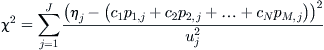 (4.45)
where ![]() is the variance of the difference
is the variance of the difference ![]() given by:
given by:
![]() (4.46)
(4.46)
As can be understood from above, to find coefficients c1, c2, …, cM and their standard uncertainties by minimizing χ2 function is complicated, because of the non-linearity present in Eq. (4.45). A possible way to do it easily is to find these uncertainties numerically as follows (Press et al., 1996):
Let K be a matrix whose N × M components ki,j are constructed from M basic functions evaluated at the N experimental values of ![]() and
and ![]() , weighted by the uncertainty ui:
, weighted by the uncertainty ui:

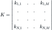 (4.47)
Let also L be a vector of length N whose components li are constructed from values of ηi to be fitted, weighted by the uncertainty ui:
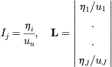 (4.48)
The normal equation of the least square problem can be written as follows:
![]() (4.49)
(4.49)
where C is a vector whose elements are the fitted coefficients.
For the calculation of variances ![]() the knowledge of coefficients c1, c2, …, cM is needed, so a possible solution is to use the values of coefficients calculated by standard least squares fitting as the initial values. These initial values can be used in Eq. (4.46) for the calculation of
the knowledge of coefficients c1, c2, …, cM is needed, so a possible solution is to use the values of coefficients calculated by standard least squares fitting as the initial values. These initial values can be used in Eq. (4.46) for the calculation of ![]() , I = 1, …, I and the formation of matrix K and of vector L.
, I = 1, …, I and the formation of matrix K and of vector L.
The solution of Eq. (4.49) gives the new values of coefficients c1, c2, …, cM, which are not expected to differ noticeably from those calculated by standard least squares fitting and used as initial values for the calculation of ![]() .
.
Furthermore, if Z = INV(KT·K) is a matrix whose diagonal elements zk,k are the squared uncertainties (variances) and the off-diagonal elements zk,l = zl,k, for k ≠ l are the covariance between fitted coefficients:
![]() (4.50)
(4.50)
where
![]() (4.51)
(4.51)
The knowledge of covariance between the fitted coefficients is necessary if one wishes to calculate, in a next stage, the uncertainty u(η) in the predicted values of η using Eqs (4.39) and (4.44).
It should be noted that Eq. (4.49) can be solved by a standard numerical method (e.g. Gauss–Jordan elimination). It is also possible to use matrix manipulation functions of spreadsheets.
For a more detailed review of the different aspects of determination of uncertainties in solar collector testing see also Mathioulakis et al. (1999), Müller-Schöll and Frei (2000), and Sabatelli et al. (2002).
Leave a Reply