
Another test required for the concentrating collectors is the determination of the collector acceptance angle, which characterizes the effect of errors in the tracking mechanism angular orientation.
This can be found with the tracking mechanism disengaged and by measuring the efficiency at various out-of-focus angles as the sun is traveling over the collector plane. An example is shown in Figure 4.8, where the angle of incidence measured from the normal to the tracking axis (i.e., out-of-focus angle) is plotted against the efficiency factor, that is, the ratio of the maximum efficiency at normal incidence to the efficiency at a particular out-of-focus angle.
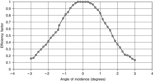
FIGURE 4.8 Parabolic trough collector acceptance angle test results.
A definition of the collector acceptance angle is the range of incidence angles (as measured from the normal to the tracking axis) in which the efficiency factor varies by no more than 2% from the value of normal incidence (ASHRAE, 2010). Therefore, from Figure 4.8, the collector half acceptance angle, θm, is 0.5°. This angle determines the maximum error of the tracking mechanism.
4.4 Collector time constant
A last aspect of collector testing is the determination of the heat capacity of a collector in terms of a time constant. It is also necessary to determine the time response of the solar collector to be able to evaluate the transient behavior of the collector and select the correct time intervals for the quasi-steady-state or steady-state efficiency tests. Whenever transient conditions exist, Eqs (4.9)–(4.14) do not govern the thermal performance of the collector, since part of the absorbed solar energy is used for heating up the collector and its components.
The time constant of a collector is the time required for the fluid leaving the collector to reach 63.2% of its ultimate steady value after a step change in incident radiation. The collector time constant is a measure of the time required for the following relationship to apply (ASHRAE, 2010):
![]() (4.32)
(4.32)
Tot = collector outlet water temperature after time t (°C).
Tof = collector outlet final water temperature (°C).
Ti = collector inlet water temperature (°C).
The procedure for performing this test is as follows. The heat transfer fluid is circulated through the collector at the same flow rate as that used during collector thermal efficiency tests. The aperture of the collector is shielded from the solar radiation by means of a solar reflecting cover, or in the case of a concentrating collector, the collector is defocused and the temperature of the heat transfer fluid at the collector inlet is set approximately equal to the ambient air temperature. When a steady state has been reached, the cover is removed and measurements continue until steady-state conditions are achieved again. For the purpose of this test, a steady-state condition is assumed to exist when the outlet temperature of the fluid varies by less than 0.05 °C per minute (ISO, 1994).
The difference between the temperature of the fluid at the collector outlet at time t and that of the surrounding air (Tot − Ta) (note that, for this test, Ti = Ta) is plotted against time, beginning with the initial steady-state condition (Toi − Ta) and continuing until the second steady state has been achieved at a higher temperature (Tof − Ta), as shown in Figure 4.9.
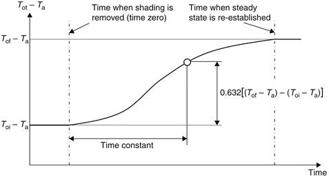
FIGURE 4.9 Time constant as specified in ISO 9806-1:1994.
The time constant of the collector is defined as the time taken for the collector outlet temperature to rise by 63.2% of the total increase from (Toi − Ta) to (Tof − Ta) following the step increase in solar irradiance at time 0.
The time constant specified in the standard ISO 9806-1:1994, as described previously, occurs when the collector warms up. Another way to perform this test, specified in ASHRAE Standard 93:2010 and carried out in addition to the preceding procedure by some researchers, is to measure the time constant during cool-down. In this case, again, the collector is operated with the fluid inlet temperature maintained at the ambient temperature. The incident solar energy is then abruptly reduced to 0 by either shielding an FPC or defocusing a concentrating one. The temperatures of the transfer fluid are continuously monitored as a function of time until Eq. (4.33) is satisfied:
![]() (4.33)
(4.33)
Toi = collector outlet initial water temperature (°C).
The graph of the difference between the various temperatures of the fluid in this case is as shown in Figure 4.10.
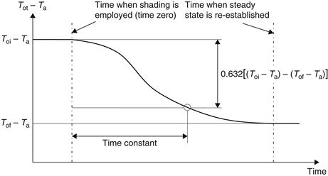
FIGURE 4.10 Time constant as specified in ASHRAE 93:2010.
The time constant of the collector, in this case, is the time taken for the collector outlet temperature to drop by 63.2% of the total increase from (Toi − Ta) to (Tof − Ta) following the step decrease in solar irradiance at time 0 (ASHRAE, 2010).
Leave a Reply