
As we have seen in Section 3.2, concentrating collectors work by interposing an optical device between the source of radiation and the energy-absorbing surface. Therefore, for concentrating collectors, both optical and thermal analyses are required. In this book, only two types of concentrating collectors are analyzed: compound parabolic and parabolic trough collectors. Initially, the concentration ratio and its theoretical maximum value are defined.
The concentration ratio (C) is defined as the ratio of the aperture area to the receiver–absorber area; that is,
![]() (3.87)
(3.87)
For FPCs with no reflectors, C = 1. For concentrators, C is always greater than 1. Initially the maximum possible concentration ratio is investigated. Consider a circular (three-dimensional) concentrator with aperture Aa and receiver area Ar located at a distance R from the center of the sun, as shown in Figure 3.35. We saw in Chapter 2 that the sun cannot be considered a point source but a sphere of radius r; therefore, as seen from the earth, the sun has a half angle, θm, which is the acceptance half angle for maximum concentration. If both the sun and the receiver are considered to be blackbodies at temperatures Ts and Tr, the amount of radiation emitted by the sun is given by:
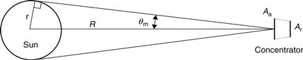
FIGURE 3.35 Schematic of the sun and a concentrator.
A fraction of this radiation is intercepted by the collector, given by:
![]() (3.89)
(3.89)
Therefore, the energy radiated from the sun and received by the concentrator is:
![]() (3.90)
(3.90)
A blackbody (perfect) receiver radiates energy equal to ![]() and a fraction of this reaches the sun, given by:
and a fraction of this reaches the sun, given by:
![]() (3.91)
(3.91)
Under this idealized condition, the maximum temperature of the receiver is equal to that of the sun. According to the second law of thermodynamics, this is true only when Qr–s = Qs–r. Therefore, from Eqs (3.90) and (3.91),
![]() (3.92)
(3.92)
Since the maximum value of Fr–s is equal to 1, the maximum concentration ratio for three-dimensional concentrators is [sin(θm) = r/R]:
![]() (3.93)
(3.93)
A similar analysis for linear concentrators gives:
![]() (3.94)
(3.94)
As was seen in Chapter 2, 2θm is equal to 0.53° (or 32′), so θm, the half acceptance angle, is equal to 0.27° (or 16′). The half acceptance angle denotes coverage of one half of the angular zone within which radiation is accepted by the concentrator’s receiver. Radiation is accepted over an angle of 2θm, because radiation incident within this angle reaches the receiver after passing through the aperture. This angle describes the angular field within which radiation can be collected by the receiver without having to track the concentrator.
Equations (3.93) and (3.94) define the upper limit of concentration that may be obtained for a given collector viewing angle. For a stationary CPC, the angle θm depends on the motion of the sun in the sky. For a CPC having its axis in an N–S direction and tilted from the horizontal such that the plane of the sun’s motion is normal to the aperture, the acceptance angle is related to the range of hours over which sunshine collection is required; for example, for 6 h of useful sunshine collection, 2θm = 90° (sun travels 15°/h). In this case, Cmax = 1/sin(45°) = 1.41.
For a tracking collector, θm is limited by the size of the sun’s disk, small-scale errors, irregularities of the reflector surface, and tracking errors. For a perfect collector and tracking system, Cmax depends only on the sun’s disk. Therefore,
For single-axis tracking, Cmax = 1/sin(16′) = 216.
For full tracking, Cmax = 1/sin2(16′) = 46,747.
It can therefore be concluded that the maximum concentration ratio for two-axis tracking collectors is much higher. However, high accuracy of the tracking mechanism and careful construction of the collector are required with an increased concentration ratio, because θm is very small. In practice, due to various errors, much lower values than these maximum ones are employed.
EXAMPLE 3.7
From the diameter of the sun and the earth and the mean distance of sun from earth, shown in Figure 2.1, estimate the amount of energy emitted from the sun, the amount of energy received by the earth, and the solar constant for a sun temperature of 5777 K. If the distance of Venus from the sun is 0.71 times the mean sun–earth distance, estimate the solar constant for Venus.
Solution
The amount of energy emitted from the sun, Qs, is:

or

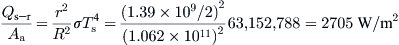
From Eq. (3.90), the solar constant can be obtained as:
The area of the earth exposed to sunshine is πd2/4. Therefore, the amount of energy received from earth = π(1.27 × 10⁷)2 × 1.363/4 = 1.73 × 10¹⁴ kW. These results verify the values specified in the introduction to Chapter 2.
The mean distance of Venus from the sun is 1.496 × 1011 × 0.71 = 1.062 × 10¹¹ m. Therefore, the solar constant of Venus is:
3.6.1 Optical analysis of a compound parabolic collector
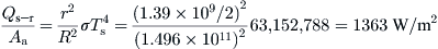
The optical analysis of CPC collectors deals mainly with the way to construct the collector shape. A CPC of the Winston design (Winston and Hinterberger, 1975) is shown in Figure 3.36. It is a linear two-dimensional concentrator consisting of two distinct parabolas, the axes of which are inclined at angles ±θc with respect to the optical axis of the collector. The angle θc, called the collector half acceptance angle, is defined as the angle through which a source of light can be moved and still converge at the absorber.
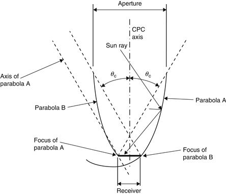
FIGURE 3.36 Construction of a flat receiver compound parabolic collector.
The Winston-type collector is a non-imaging concentrator with a concentration ratio approaching the upper limit permitted by the second law of thermodynamics, as explained in previous section.
The receiver of the CPC does not have to be flat and parallel but, as shown in Figure 3.5, can be bifacial, a wedge, or cylindrical. Figure 3.37 shows a collector with a cylindrical receiver; the lower portion of the reflector (AB and AC) is circular, while the upper portions (BD and CE) are parabolic. In this design, the requirement for the parabolic portion of the collector is that, at any point P, the normal to the collector must bisect the angle between the tangent line PG to the receiver and the incident ray at point P at angle θc with respect to the collector axis. Since the upper part of a CPC contributes little to the radiation reaching the absorber, it is usually truncated, forming a shorter version of the CPC, which is also cheaper. CPCs are usually covered with glass to avoid dust and other materials entering the collector and reducing the reflectivity of its walls. Truncation hardly affects the acceptance angle but results in considerable material saving and changes the height-to-aperture ratio, the concentration ratio, and the average number of reflections.
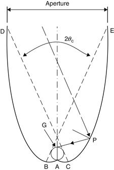
FIGURE 3.37 Schematic diagram of a CPC collector.
These collectors are more useful as linear or trough-type concentrators. The orientation of a CPC collector is related to its acceptance angle (2θc, in Figures 3.36 and 3.37). The two-dimensional CPC is an ideal concentrator, that is, it works perfectly for all rays within the acceptance angle, 2θc. Also, depending on the collector acceptance angle, the collector can be stationary or tracking. A CPC concentrator can be oriented with its long axis along either the north–south or east–west direction and its aperture tilted directly toward the equator at an angle equal to the local latitude. When oriented along the north–south direction, the collector must track the sun by turning its axis to face the sun continuously. Since the acceptance angle of the concentrator along its long axis is wide, seasonal tilt adjustment is not necessary. It can also be stationary, but radiation will be received only during the hours when the sun is within the collector acceptance angle.
When the concentrator is oriented with its long axis along the east–west direction, with a little seasonal adjustment in tilt angle, the collector is able to catch the sun’s rays effectively through its wide acceptance angle along its long axis. The minimum acceptance angle in this case should be equal to the maximum incidence angle projected in a north–south vertical plane during the times when output is needed from the collector. For stationary CPC collectors mounted in this mode, the minimum acceptance angle is equal to 47°. This angle covers the declination of the sun from summer to winter solstices (2 × 23.5°). In practice, bigger angles are used to enable the collector to collect diffuse radiation at the expense of a lower concentration ratio. Smaller (less than 3) concentration ratio CPCs are of greatest practical interest. These, according to Pereira (1985), are able to accept a large proportion of diffuse radiation incident on their apertures and concentrate it without the need to track the sun. Finally, the required frequency of collector adjustment is related to the collector concentration ratio. Thus, for C ≤ 3 the collector needs only biannual adjustment, while for C > 10 the collector requires almost daily adjustment; these systems are also called quasi-static.
Concentrators of the type shown in Figure 3.5 have an area concentration ratio that is a function of the acceptance half angle, θc. For an ideal linear concentrator system, this is given by Eq. (3.94) by replacing θm with θc.
3.6.2 Thermal analysis of compound parabolic collectors
The instantaneous efficiency, η, of a CPC is defined as the useful energy gain divided by the incident radiation on the aperture plane; that is,
![]() (3.95)
(3.95)
In Eq. (3.95), Gt is the total incident radiation on the aperture plane. The useful energy, Qu, is given by an equation similar to Eq. (3.60), using the concept of absorbed radiation as:
![]() (3.96)
(3.96)
The absorbed radiation, S, is obtained from (Duffie and Beckman, 2006):
![]() (3.97)
(3.97)
τc = transmittance of the CPC cover.
τCPC = transmissivity of the CPC to account for reflection loss.
The various radiation components in Eq. (3.97) come from radiation falling on the aperture within the acceptance angle of the CPC and are given as follows:
![]() (3.98a)
(3.98a)
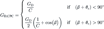 (3.98b)
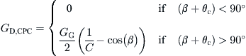 (3.98c)
In Eqs (3.98a)–(3.98c), β is the collector aperture inclination angle with respect to horizontal. In Eq. (3.98c), the ground-reflected radiation is effective only if the collector receiver “sees” the ground, that is, (β + θc) > 90°.
It has been shown by Rabl et al. (1980) that the insolation, GCPC, of a collector with a concentration C can be approximated very well from:
![]() (3.99)
(3.99)
It is convenient to express the absorbed solar radiation, S, in terms of GCPC in the following way:
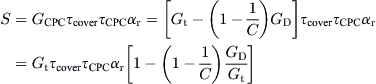 (3.100)
or
![]() (3.101)
(3.101)
τcover = transmissivity of the cover glazing.
τCPC = effective transmissivity of CPC.
αr = absorptivity of receiver.
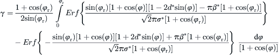
γ = correction factor for diffuse radiation, given by:
![]() (3.102)
(3.102)
The factor γ, given by Eq. (3.102), accounts for the loss of diffuse radiation outside the acceptance angle of the CPC with a concentration C. The ratio GD/Gt varies from about 0.11 on very clear sunny days to about 0.23 on hazy days.
It should be noted that only part of the diffuse radiation effectively enters the CPC, and this is a function of the acceptance angle. For isotropic diffuse radiation, the relationship between the effective incidence angle and the acceptance half angle is given by (Brandemuehl and Beckman, 1980):
![]() (3.103)
(3.103)
The effective transmissivity, τCPC, of the CPC accounts for reflection loss inside the collector. The fraction of the radiation passing through the collector aperture and eventually reaching the absorber depends on the specular reflectivity, ρ, of the CPC walls and the average number of reflections, n, expressed approximately by:
![]() (3.104)
(3.104)
This equation can also be used to estimate τCPC,B, τCPC,D, and τCPC,G in Eq. (3.97), which are usually treated as the same. Values of n for full and truncated CPCs can be obtained from Figure 3.38. As noted before, the upper ends of CPCs contribute little to the radiation reaching the receiver, and usually CPCs are truncated for economic reasons. As can be seen from Figure 3.38, the average number of reflections is a function of concentration ratio, C, and the acceptance half angle, θc. For a truncated concentrator, the line (1 − 1/C) can be taken as the lower bound for the number of reflections for radiation within the acceptance angle. Other effects of truncation are shown in Figures 3.39 and 3.40. Figures 3.38–3.40 can be used to design a CPC, as shown in the following example. For more accuracy, the equations representing the curves of Figures 3.38–3.40 can be used as given in Appendix 6.
EXAMPLE 3.8
Find the CPC characteristics for a collector with acceptance half angle θc = 12°. Find also its characteristics if the collector is truncated so that its height-to-aperture ratio is 1.4.
Solution
For a full CPC, from Figure 3.39 for θc = 12°, the height-to-aperture ratio = 2.8 and the concentration ratio = 4.8. From Figure 3.40, the area of the reflector is 5.6 times the aperture area; and from Figure 3.38, the average number of reflections of radiation before reaching the absorber is 0.97.
For a truncated CPC, the height-to-aperture ratio = 1.4. Then, from Figure 3.39, the concentration ratio drops to 4.2; and from Figure 3.40, the reflector-to-aperture area drops to 3, which indicates how significant is the saving in reflector material. Finally, from Figure 3.38, the average number of reflections is at least 1 − 1/4.2 = 0.76.
EXAMPLE 3.9
A CPC has an aperture area of 4 m2 and a concentration ratio of 1.7. Estimate the collector efficiency given the following:
Diffuse to total radiation ratio = 0.12.
Glass cover transmissivity = 0.90.
Collector heat loss coefficient = 2.5 W/m2 K.
Entering fluid temperature = 80 °C.
Collector efficiency factor = 0.92.
Solution
The diffuse radiation correction factor, γ, is estimated from Eq. (3.102):
From Figure 3.38 for C = 1.7, the average number of reflections for a full CPC is n = 0.6. Therefore, from Eq. (3.104),
The absorber radiation is given by Eq. (3.101):

The heat removal factor is estimated from Eq. (3.58):

The receiver area is obtained from Eq. (3.87):

The useful energy gain can be estimated from Eq. (3.96):

The collector efficiency is given by Eq. (3.95):
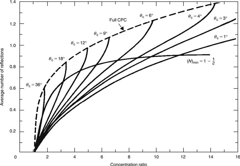
FIGURE 3.38 Average number of reflections for full and truncated CPCs. Reprinted from Rabl (1976) with permission from Elsevier.
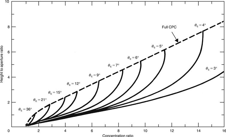
FIGURE 3.39 Ratio of height to aperture for full and truncated CPCs. Reprinted from Rabl (1976) with permission from Elsevier.
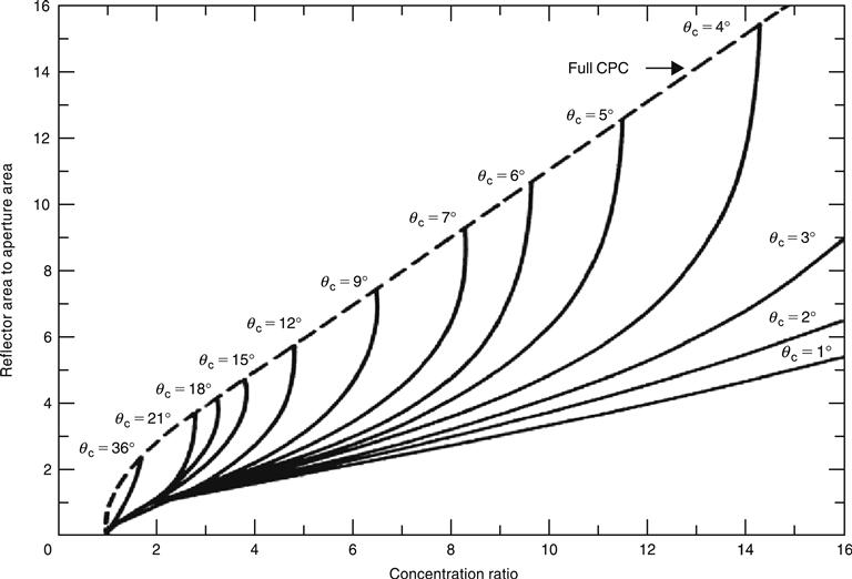
FIGURE 3.40 Ratio of reflector to aperture area for full and truncated CPCs. Reprinted from Rabl (1976) with permission from Elsevier.
3.6.3 Optical analysis of parabolic trough collectors
A cross-section of a parabolic trough collector is shown in Figure 3.41, where various important factors are shown. The incident radiation on the reflector at the rim of the collector (where the mirror radius, rr, is maximum) makes an angle, φr, with the center line of the collector, which is called the rim angle. The equation of the parabola in terms of the coordinate system is:
![]() (3.105)
(3.105)
where f = parabola focal distance (m).
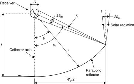
FIGURE 3.41 Cross-section of a parabolic trough collector with circular receiver.
For specular reflectors of perfect alignment, the size of the receiver (diameter D) required to intercept all the solar image can be obtained from trigonometry and Figure 3.41, given by:
![]() (3.106)
(3.106)
θm = half acceptance angle (degrees).
For a parabolic reflector, the radius, r, shown in Figure 3.41 is given by:
![]() (3.107)
(3.107)
φ = angle between the collector axis and a reflected beam at the focus; see Figure 3.41.
As φ varies from 0 to φr, r increases from f to rr and the theoretical image size increases from 2f sin(θm) to 2rr sin(θm)/cos(φr + θm). Therefore, there is an image spreading on a plane normal to the axis of the parabola.
At the rim angle, φr, Eq. (3.107) becomes:
![]() (3.108)
(3.108)
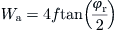
Another important parameter related to the rim angle is the aperture of the parabola, Wa. From Figure 3.41 and simple trigonometry, it can be found that:
![]() (3.109)
(3.109)
Substituting Eq. (3.108) into Eq. (3.109) gives:
![]() (3.110)
(3.110)
which reduces to:
![]() (3.111)
(3.111)
The half acceptance angle, θm, used in Eq. (3.106) depends on the accuracy of the tracking mechanism and the irregularities of the reflector surface. The smaller these two effects, the closer θm is to the sun disk angle, resulting in a smaller image and higher concentration. Therefore, the image width depends on the magnitude of the two quantities. In Figure 3.41, a perfect collector is assumed and the solar beam is shown striking the collector at an angle 2θm and leaving at the same angle. In a practical collector, however, because of the presence of errors, the angle 2θm should be increased to include the errors as well. Enlarged images can also result from the tracking mode used to transverse the collector. Problems can also arise due to errors in the positioning of the receiver relative to the reflector, which results in distortion, enlargement, and displacement of the image. All these are accounted for by the intercept factor, which is explained later in this section.
For a tubular receiver, the concentration ratio is given by:
![]() (3.112)
(3.112)
By replacing D and Wa with Eqs (3.106) and (3.110), respectively, we get:
![]() (3.113)
(3.113)
The maximum concentration ratio occurs when φr is 90° and sin(φr) = 1. Therefore, by replacing sin(φr) = 1 in Eq. (3.113), the following maximum value can be obtained:
![]() (3.114)
(3.114)
The difference between this equation and Eq. (3.94) is that this one applies particularly to a PTC with a circular receiver, whereas Eq. (3.94) is the idealized case. So, by using the same sun half acceptance angle of 16′ for single-axis tracking, Cmax = 1/πsin(16′) = 67.5.
In fact, the magnitude of the rim angle determines the material required for the construction of the parabolic surface. The curve length of the reflective surface is given by:
![]() (3.115)
(3.115)
Hp = lactus rectum of the parabola (m). This is the opening of the parabola at the focal point.
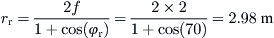
As shown in Figure 3.42 for the same aperture, various rim angles are possible. It is also shown that, for different rim angles, the focus-to-aperture ratio, which defines the curvature of the parabola, changes. It can be demonstrated that, with a 90° rim angle, the mean focus-to-reflector distance and hence the reflected beam spread is minimized, so that the slope and tracking errors are less pronounced. The collector’s surface area, however, decreases as the rim angle is decreased. There is thus a temptation to use smaller rim angles because the sacrifice in optical efficiency is small, but the saving in reflective material cost is great.
EXAMPLE 3.10
For a PTC with a rim angle of 70°, aperture of 5.6 m, and receiver diameter of 50 mm, estimate the focal distance, the concentration ratio, the rim radius, and the length of the parabolic surface.
Solution
From Eq. (3.111),
Therefore,
From Eq. (3.112), the concentration ratio is:

The rim radius is given by Eq. (3.108):
The parabola lactus rectum, Hp, is equal to Wa at φr = 90° and f = 2 m. From Eq. (3.111),

Finally, the length of the parabola can be obtained from Eq. (3.115) by recalling that sec(x) = 1/cos(x):

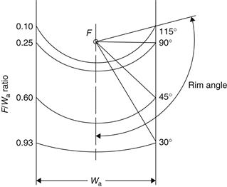
FIGURE 3.42 Parabola focal length and curvature.
Optical efficiency
Optical efficiency is defined as the ratio of the energy absorbed by the receiver to the energy incident on the collector’s aperture. The optical efficiency depends on the optical properties of the materials involved, the geometry of the collector, and the various imperfections arising from the construction of the collector. In equation form (Sodha et al., 1984):
![]() (3.116)
(3.116)
ρ = reflectance of the mirror.
τ = transmittance of the glass cover.
α = absorptance of the receiver.
The geometry of the collector dictates the geometric factor, Af, which is a measure of the effective reduction of the aperture area due to abnormal incidence effects, including blockages, shadows, and loss of radiation reflected from the mirror beyond the end of the receiver. During abnormal operation of a PTC, some of the rays reflected from near the end of the concentrator opposite the sun cannot reach the receiver. This is called the end effect. The amount of aperture area lost is shown in Figure 3.43 and given by:
![]() (3.117)
(3.117)
Usually, collectors of this type are terminated with opaque plates to preclude unwanted or dangerous concentration away from the receiver. These plates result in blockage or shading of a part of the reflector, which in effect reduces the aperture area. For a plate extending from rim to rim, the lost area is shown in Figure 3.43 and given by:
![]() (3.118)
(3.118)
It should be noted that the term tan(θ) shown in Eqs (3.117) and (3.118) is the same as the one shown in Eq. (3.116), and it should not be used twice. Therefore, to find the total loss in aperture area, Al, the two areas, Ae and Ab, are added together without including the term tan(θ) (Jeter, 1983):
![]() (3.119)
(3.119)
Finally, the geometric factor is the ratio of the lost area to the aperture area. Therefore,
![]() (3.120)
(3.120)
The most complex parameter involved in determining the optical efficiency of a PTC is the intercept factor. This is defined as the ratio of the energy intercepted by the receiver to the energy reflected by the focusing device, that is, the parabola. Its value depends on the size of the receiver, the surface angle errors of the parabolic mirror, and the solar beam spread.
FIGURE 3.43 End effect and blocking in a parabolic trough collector.
The errors associated with the parabolic surface are of two types: random and non-random (Guven and Bannerot, 1985). Random errors are defined as those errors that are truly random in nature and, therefore, can be represented by normal probability distributions. Random errors are identified as apparent changes in the sun’s width, scattering effects caused by random slope errors (i.e., distortion of the parabola due to wind loading), and scattering effects associated with the reflective surface. Non-random errors arise in manufacture assembly or the operation of the collector. These can be identified as reflector profile imperfections, misalignment errors, and receiver location errors. Random errors are modeled statistically, by determining the standard deviation of the total reflected energy distribution, at normal incidence (Guven and Bannerot, 1986), and are given by:
![]() (3.121)
(3.121)
Non-random errors are determined from a knowledge of the misalignment angle error β (i.e., the angle between the reflected ray from the center of the sun and the normal to the reflector’s aperture plane) and the displacement of the receiver from the focus of the parabola (dr). Since reflector profile errors and receiver mislocation along the Y axis essentially have the same effect, a single parameter is used to account for both. According to Guven and Bannerot (1986), random and non-random errors can be combined with the collector geometric parameters, concentration ratio (C), and receiver diameter (D) to yield error parameters universal to all collector geometries. These are called universal error parameters, and an asterisk is used to distinguish them from the already defined parameters. Using the universal error parameters, the formulation of the intercept factor, γ, is possible (Guven and Bannerot, 1985):
 (3.122)
d∗ = universal non-random error parameter due to receiver mislocation and reflector profile errors, d∗ = dr/D.
β∗ = universal non-random error parameter due to angular errors, β∗ = βC.
σ∗ = universal random error parameter, σ∗ = σC.
C = collector concentration ratio, = Aa/Ar.
D = riser tube outside diameter (m).
dr = displacement of receiver from focus (m).
β = misalignment angle error (degrees).
Another type of analysis commonly carried out in concentrating collectors is ray tracing. This is the process of following the paths of a large number of rays of incident radiation through the optical system to determine the distribution and intensity of the rays on the surface of the receiver. Ray tracing determines the radiation concentration distribution on the receiver of the collector, called the local concentration ratio (LCR). As was seen in Figure 3.41, the radiation incident on a differential element of reflector area is a cone having a half angle of 16′. The reflected radiation is a similar cone, having the same apex angle if the reflector is perfect. The intersection of this cone with the receiver surface determines the image size and shape for that element, and the total image is the sum of the images for all the elements of the reflector. In an actual collector, the various errors outlined previously, which enlarge the image size and lower the LCR, are considered. The distribution of the LCR for a parabolic trough collector is shown in Figure 3.44. The shape of the curves depends on the random and non-random errors mentioned above and on the angle of incidence. It should be noted that the distribution for half of the receiver is shown in Figure 3.44. Another more representative way to show this distribution for the whole receiver is in Figure 3.45. As can be seen , the top part of the receiver essentially receives only direct sunshine from the sun and the maximum concentration for this particular collector, about 36 suns, occurs at 0 incidence angle and at an angle β of 120° (Figure 3.44).
EXAMPLE 3.11
For a PTC with a total aperture area of 50 m2, aperture of 2.5 m, and rim angle of 90°, estimate the geometric factor and the actual area lost at an angle of incidence equal to 60°.
Solution
As φr = 90°, the parabola height hp = f. Therefore, from Eq. (3.111),
From Eq. (3.119):

The area lost at an incidence angle of 60° is:

The geometric factor Af is obtained from Eq. (3.120):
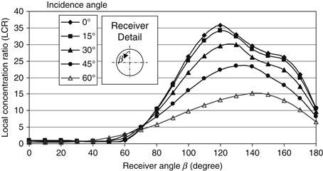
FIGURE 3.44 Local concentration ratio on the receiver of a parabolic trough collector.
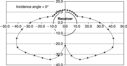
FIGURE 3.45 A more representative view of LCR for a collector with receiver diameter of 20 mm and rim angle of 90°.
3.6.4 Thermal analysis of parabolic trough collectors
The generalized thermal analysis of a concentrating solar collector is similar to that of a flat-plate collector. It is necessary to derive appropriate expressions for the collector efficiency factor, F′; the loss coefficient, UL; and the collector heat removal factor, FR. For the loss coefficient, standard heat transfer relations for glazed tubes can be used. Thermal losses from the receiver must be estimated, usually in terms of the loss coefficient, UL, which is based on the area of the receiver. The method for calculating thermal losses from concentrating collector receivers cannot be as easily summarized as for the flat-plate ones, because many designs and configurations are available. Two such designs are presented in this book: the PTC with a bare tube and the glazed tube receiver. In both cases, the calculations must include radiation, conduction, and convection losses.
For a bare tube receiver and assuming no temperature gradients along the receiver, the loss coefficient considering convection and radiation from the surface and conduction through the support structure is given by:
The linearized radiation coefficient can be estimated from:
![]() (3.124)
(3.124)
If a single value of hr is not acceptable due to large temperature variations along the flow direction, the collector can be divided into small segments, each with a constant hr.
For the wind loss coefficient, the Nusselt number can be used.
For 0.1 < Re < 1000,
![]() (3.125a)
(3.125a)
For 1000 < Re < 50,000,
![]() (3.125b)
(3.125b)
Estimation of the conduction losses requires knowledge of the construction of the collector, that is, the way the receiver is supported.
Usually, to reduce the heat losses, a concentric glass tube is employed around the receiver. The space between the receiver and the glass is usually evacuated, in which case the convection losses are negligible. In this case, UL, based on the receiver area Ar, is given by:
![]() (3.126)
(3.126)
hr,c–a = linearized radiation coefficient from cover to ambient estimated by Eq. (3.124) (W/m2 K).
Ag = external area of glass cover (m2).
hr,r–c = linearized radiation coefficient from receiver to cover, given by Eq. (2.74):
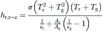 (3.127)
In the preceding equations, to estimate the glass cover properties, the temperature of the glass cover, Tg, is required. This temperature is closer to the ambient temperature than the receiver temperature. Therefore, by ignoring the radiation absorbed by the cover, Tg may be obtained from an energy balance:
![]() (3.128)
(3.128)
Solving Eq. (3.128) for Tg gives:
![]() (3.129)
(3.129)
The procedure to find Tg is by iteration, that is, estimate UL from Eq. (3.126) by considering a random Tg (close to Ta). Then, if Tg obtained from Eq. (3.129) differs from original value, iterate. Usually, no more than two iterations are required.
If radiation absorbed by the cover needs to be considered, the appropriate term must be added to the right-hand side of Eq. (3.126). The principles are the same as those developed earlier for the flat-plate collectors.
Next, the overall heat transfer coefficient, Uo, needs to be estimated. This should include the tube wall because the heat flux in a concentrating collector is high. Based on the outside tube diameter, this is given by:
![]() (3.130)
(3.130)
Do = receiver outside tube diameter (m).
Di = receiver inside tube diameter (m).
hfi = convective heat transfer coefficient inside the receiver tube (W/m2 K).
The convective heat transfer coefficient, hfi, can be obtained from the standard pipe flow equation:
![]() (3.131)
(3.131)
Re = Reynolds number = ρVDi/μ.
kf = thermal conductivity of fluid (W/m K).
It should be noted that Eq. (3.131) is for turbulent flow (Re > 2300). For laminar flow, Nu = 4.364 = constant.
A detailed thermal model of a PTC is presented by Kalogirou (2012). In this all modes of heat transfer were considered in detail and the set of equations obtained were solved simultaneously. For this purpose the program Engineering Equation Solver (EES) is used which includes routines to estimate the properties of various substances and can be called from TRNSYS (see Chapter 11, Section 11.5.1) which allows the development of a model that can use the capabilities of both programs.
The instantaneous efficiency of a concentrating collector may be calculated from an energy balance of its receiver. Equation (3.31) also may be adapted for use with concentrating collectors by using appropriate areas for the absorbed solar radiation (Aa) and heat losses (Ar). Therefore, the useful energy delivered from a concentrator is:
![]() (3.132)
(3.132)
Note that, because concentrating collectors can utilize only beam radiation, GB is used in Eq. (3.132) instead of the total radiation, Gt, used in Eq. (3.31).
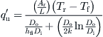
The useful energy gain per unit of collector length can be expressed in terms of the local receiver temperature, Tr, as:
![]() (3.133)
(3.133)
In terms of the energy transfer to the fluid at the local fluid temperature, Tf (Kalogirou, 2004),
 (3.134)
If Tr is eliminated from Eqs (3.133) and (3.134), we have:
![]() (3.135)
(3.135)
where F′ is the collector efficiency factor, given by:
![]() (3.136)
(3.136)
As for the flat-plate collector, Tr in Eq. (3.132) can be replaced by Ti through the use of the heat removal factor, and Eq. (3.132) can be written as:
![]() (3.137)
(3.137)
The collector efficiency can be obtained by dividing Qu by (GBAa). Therefore,
![]() (3.138)
(3.138)
C = concentration ratio, C = Aa/Ar.
For FR, a relation similar to Eq. (3.58) is used by replacing Ac with Ar and using F′, given by Eq. (3.136), which does not include the fin and bond conductance terms, as in FPCs. This equation explains why high temperatures can be obtained with concentrating collectors. This is because the heat losses term is inversely proportional to C, so the bigger the concentration ratio the smaller the losses.
Consideration of vacuum in annulus space
In the analysis presented so far, the convection losses in the annulus space are ignored. In fact convection heat transfer depends on the annulus pressure. At low pressures (<0.013 Pa), heat transfer is by molecular conduction, whereas at higher pressures is by free convection. When the annulus is under vacuum (pressure <0.013 Pa), the convection heat transfer between the receiver pipe and glass envelope occurs by free molecular convection and the heat transfer coefficient is given by (Ratzel et al., 1979):
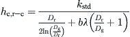 (3.139)
This equation is applicable for: Ra < (Dg/(Dg − Dr))4.
And
![]() (3.140)
(3.140)
![]() (3.141)
(3.141)
kstd = thermal conductivity of the annulus gas at standard temperature and pressure (W/m °C)
Dr = outside receiver pipe diameter (m)
Dg = inside glass envelope diameter (m)
λ = mean free path between collisions of a molecule (cm)
γ = ratio of specific heats for the annulus gas (air)
Tr–g = average temperature (Tr + Tg)/2 (°C)
Pa = annulus gas pressure (mmHg) and
δ = molecular diameter of annulus gas (cm).
Equation (3.139) slightly overestimates the heat transfer for very small pressures (<0.013 Pa). The molecular diameters of air, δ, is equal to 3.55 × 10⁻⁸ cm (Marshal, 1976), the thermal conductivity of air is 0.02551 W/m °C, the interaction coefficient is 1.571, the mean free path between collisions of a molecule is 88.67 cm, and the ratio of specific heats for the annulus air is 1.39. These are for average fluid temperature of 300 °C and pressure equal to 0.013 Pa. Using these values, the convection heat transfer coefficient (hc,r–c) is equal to 0.0001115 W/m2 °C, which is the reason why usually it is ignored.
If for more accuracy this heat loss is considered Eq. (3.126) should include hc,r–c in the second term as well as Eq. (3.128) for the appropriate estimation of Tg.
If the receiver is filled or partially filled with ambient air or if the receiver annulus vacuum is lost, the convection heat transfer between the receiver pipe and glass envelope occurs by natural convection and for this purpose, the correlation for natural convection in an annular space (enclosure) between horizontal concentric cylinders can be used, found in many heat transfer books.
EXAMPLE 3.12
A 20 m long PTC with an aperture width of 3.5 m has a pipe receiver of 50 mm outside diameter and 40 mm inside diameter and a glass cover of 90 mm in diameter. If the space between the receiver and the glass cover is evacuated, estimate the overall collector heat loss coefficient, the useful energy gain, and the exit fluid temperature. The following data are given:
Absorbed solar radiation = 500 W/m2.
Receiver temperature = 260 °C = 533 K.
Receiver emissivity, εr = 0.92.
Glass cover emissivity, εg = 0.87.
Circulating fluid, cp = 1350 J/kg K.
Entering fluid temperature = 220 °C = 493 K.
Heat transfer coefficient inside the pipe = 330 W/m2 K.
Tube thermal conductivity, k = 15 W/m K.
Ambient temperature = 25 °C = 298 K.
Solution
The receiver area Ar = πDoL = π × 0.05 × 20 = 3.14 m2. The glass cover area Ag = πDgL = π × 0.09 × 20 = 5.65 m2. The unshaded collector aperture area Aa = (3.5 − 0.09) × 20 = 68.2 m2.
Next, a glass cover temperature, Tg, is assumed to evaluate the convection and radiation heat transfer from the glass cover. This is assumed to be equal to 64 °C = 337 K. The actual glass cover temperature is obtained by iteration by neglecting the interactions with the reflector. The convective (wind) heat transfer coefficient hc,c–a = hw of the glass cover can be calculated from Eq. (3.125). First, the Reynolds number needs to be estimated at the mean temperature ½(25 + 64) = 44.5 °C. Therefore, from Table A5.1 in Appendix 5, we get:
Now

Therefore, Eq. (3.125b) applies, which gives:
and

The radiation heat transfer coefficient, hr,c–a, for the glass cover to the ambient is calculated from Eq. (2.75):

The radiation heat transfer coefficient, hr,r–c, between the receiver tube and the glass cover is estimated from Eq. (3.127):
Since the space between the receiver and the glass cover is evacuated, there is no convection heat transfer. Therefore, based on the receiver area, the overall collector heat loss coefficient is given by Eq. (3.126):

Since UL is based on the assumed Tg value, we need to check if the assumption made was correct. Using Eq. (3.129), we get:

This is about the same as the value assumed earlier.
The collector efficiency factor can be calculated from Eq. (3.136):
The heat removal factor can be calculated from Eq. (3.58) by using Ar instead of Ac:

The useful energy is estimated from Eq. (3.137) using the concept of absorbed radiation:

Finally, the fluid exit temperature can be estimated from:

Another analysis usually performed for PTCs applies a piecewise two-dimensional model of the receiver by considering the circumferential variation of solar flux shown in Figures 3.44 and 3.45. Such an analysis can be performed by dividing the receiver into longitudinal and isothermal nodal sections, as shown in Figure 3.46, and applying the principle of energy balance to the glazing and receiver nodes (Karimi et al., 1986).
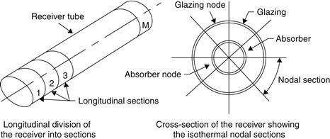
FIGURE 3.46 Piecewise two-dimensional model of the receiver assembly. Karimi et al. (1986).
The generalized glazing and absorber nodes, showing the various modes of heat transfer considered, are shown in Figure 3.47. It is assumed that the length of each section is very small so that the working fluid in that section stays in the inlet temperature. The temperature is adjusted in a stepwise fashion at the end of the longitudinal section. By applying the principle of energy balance to the glazing and absorber nodes, we get the following equations.
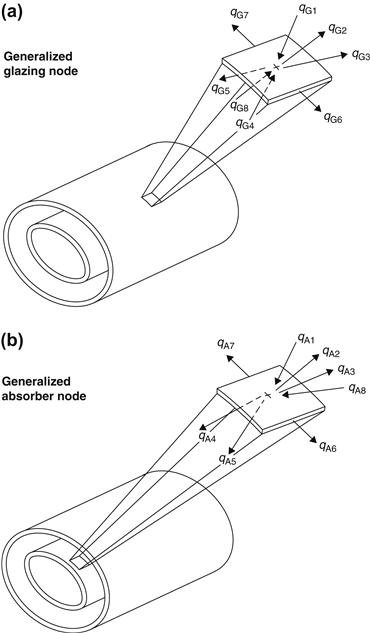
FIGURE 3.47 Generalized glazing and absorber nodes, showing the various modes of heat transfer. Karimi et al. (1986).
For the glazing node,
![]() (3.142)
(3.142)
For the absorber node,
![]() (3.143)
(3.143)
qG1 = solar radiation absorbed by glazing node i.
qG2 = net radiation exchange between glazing node i to the surroundings.
qG3 = natural and forced convection heat transfer from glazing node i to the surroundings.
qG4 = convection heat transfer to the glazing node from the absorber (across the gap).
qG5 = radiation emitted by the inside surface of the glazing node i.
qG6 = conduction along the circumference of glazing from node i to i + 1.
qG7 = conduction along the circumference of the glazing from node i to i − 1.
qG8 = fraction of the total radiation incident upon the inside glazing surface that is absorbed.
qA1 = solar radiation absorbed by absorber node i.
qA2 = thermal radiation emitted by outside surface of absorber node i.
qA3 = convection heat transfer from absorber node to glazing (across the gap).
qA4 = convection heat transfer to absorber node i from the working fluid.
qA5 = radiation exchange between the inside surface of absorber and absorber node i.
qA6 = conduction along the circumference of absorber from node i to i + 1.
qA7 = conduction along the circumference of the absorber from node i to i − 1.
qA8 = fraction of the total radiation incident upon the inside absorber node that is absorbed.
For all these parameters, standard heat transfer relations can be used. The set of non-linear equations is solved sequentially to obtain the temperature distribution of the receiver, and the solution is obtained by an iterative procedure. In Eqs (3.142) and (3.143), factors qG1 and qA1 are calculated by the optical model, whereas factor qA5 is assumed to be negligible.
This analysis can give the temperature distribution along the circumference and length of the receiver, so any points of high temperature, which might reach a temperature above the degradation temperature of the receiver selective coating, can be determined.
Leave a Reply