
Desalination can be achieved using a number of techniques. Industrial desalination technologies either use phase change or involve semi-permeable membranes to separate the solvent or some solutes. Therefore, desalination techniques may be classified into the following categories: phase change or thermal processes and membrane or single-phase processes.
All processes require a chemical pre-treatment of raw seawater to avoid scaling, foaming, corrosion, biological growth, and fouling and also require a chemical post-treatment.
In Table 8.1, the most important technologies in use are listed. In the phase change or thermal processes, the distillation of seawater is achieved by utilizing a thermal energy source. The thermal energy may be obtained from a conventional fossil fuel source, nuclear energy, or a non-conventional solar energy source or geothermal energy. In the membrane processes, electricity is used for either driving high-pressure pumps or ionization of salts contained in the seawater.
Table 8.1
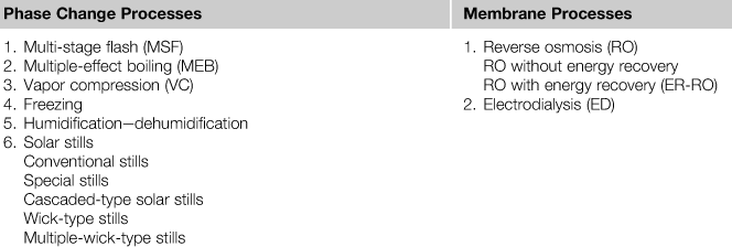
Commercial desalination processes based on thermal energy are multi-stage flash (MSF) distillation, multiple-effect boiling (MEB), and vapor compression (VC), which could be thermal vapor compression (TVC) or mechanical vapor compression (MVC). MSF and MEB processes consist of a set of stages at successively decreasing temperature and pressure. The MSF process is based on the generation of vapor from seawater or brine due to a sudden pressure reduction when seawater enters an evacuated chamber. The process is repeated stage by stage at successively decreasing pressure. This process requires an external steam supply, normally at a temperature of around 100 °C. The maximum temperature is limited by the salt concentration to avoid scaling, and this maximum limits the performance of the process. In MEB, vapors are generated through the absorption of thermal energy by the seawater. The steam generated in one stage or effect can heat the salt solution in the next effect because the next effect is at lower temperature and pressure. The performance of the MEB and MSF processes is proportional to the number of stages or effects. MEB plants normally use an external steam supply at a temperature of about 70 °C. In TVC and MVC, after the initial vapor is generated from the saline solution, it is thermally or mechanically compressed to generate additional production. More details about these processes are given in Section 8.4.
Not only distillation processes but also freezing and humidification–dehumidification processes involve phase change. The conversion of saline water to freshwater by freezing has always existed in nature and has been known to humankind for thousands of years. In desalination of water by freezing, freshwater is removed and leaves behind a concentrated brine. It is a separation process related to the solid–liquid phase change phenomenon. When the temperature of saline water is reduced to its freezing point, which is a function of salinity, ice crystals of pure water are formed within the salt solution. These ice crystals can be mechanically separated from the concentrated solution, washed, and re-melted to obtain pure water. Therefore the basic energy input for this method is for the refrigeration system (Tleimat, 1980). The humidification–dehumidification method also uses a refrigeration system, but the principle of operation is different. The humidification–dehumidification process is based on the fact that air can be mixed with large quantities of water vapor. Additionally, the vapor-carrying capability of air increases with temperature (Parekh et al., 2003). In this process, seawater is added into an air stream to increase its humidity. Then this humid air is directed to a cool coil, on the surface of which water vapor contained in the air is condensed and collected as freshwater. These processes, however, exhibit technical problems that limit their industrial development. Because these technologies have not yet industrially matured, they are not described in this chapter.
The other category of industrial desalination processes does not involve phase change but membranes. These are reverse osmosis (RO) and electrodialysis (ED). The first one requires electricity or shaft power to drive the pump that increases the pressure of the saline solution to that required. The required pressure depends on the salt concentration of the resource of saline solution, and it is normally around 70 bar for seawater desalination.
ED also requires electricity for the ionization of water, which is cleaned by using suitable membranes located at the two oppositely charged electrodes. Both RO and ED are used for brackish water desalination, but only RO competes with distillation processes in seawater desalination. The dominant processes are MSF and RO, which account for 44% and 42% of worldwide capacity, respectively (Garcia-Rodriguez, 2003). The MSF process represents more than 93% of the thermal process production, whereas the RO process represents more than 88% of membrane processes production (El-Dessouky and Ettouney, 2000). The membrane processes are described in more detail in Section 8.4.
Solar energy can be used for seawater desalination by producing either the thermal energy required to drive the phase change processes or the electricity required to drive the membrane processes. Solar desalination systems are thus classified into two categories: direct and indirect collection systems. As their name implies, direct collection systems use solar energy to produce distillate directly in the solar collector, whereas in indirect collection systems, two subsystems are employed (one for solar energy collection and one for desalination). Conventional desalination systems are similar to solar energy systems, since the same type of equipment is applied. The prime difference is that, in the former, either a conventional boiler is used to provide the required heat or public mains electricity is used to provide the required electric power; whereas in the latter, solar energy is applied. The most promising and applicable RES desalination combinations are shown in Table 8.2. These are obtained from a survey conducted under a European research project (THERMIE Program, 1998).
Table 8.2
| RES Technology | Feedwater Salinity | Desalination Technology |
| Solar thermal | Seawater Seawater | Multiple-effect boiling (MEB) Multi-stage flash (MSF) |
| Photovoltaics | Seawater Brackish water Brackish water | Reverse osmosis (RO) Reverse osmosis (RO) Electrodialysis (ED) |
| Wind energy | Seawater Brackish water Seawater | Reverse osmosis (RO) Reverse osmosis (RO) Mechanical vapor compression (MVC) |
| Geothermal | Seawater | Multiple-effect boiling (MEB) |
From 1990 to 2010, numerous desalination systems utilizing renewable energy were constructed. Almost all of these systems were built as research or demonstration projects and are consequently of a small capacity. It is not known how many of these plants still exist, but it is likely that only some remain in operation. The lessons learned, hopefully, have been passed on and are reflected in the plants currently being built and tested. A list of installed desalination plants operated with renewable energy sources is given by Tzen and Morris (2003).
8.2.1 Desalination systems exergy analysis
Although the first law of thermodynamics is an important tool in evaluating the overall performance of a desalination plant, such analysis does not take into account the quality of energy transferred. This is an issue of particular importance when both thermal and mechanical energy are employed, as they are in thermal desalination plants. First law analysis cannot show where the maximum loss of available energy takes place and would lead to the conclusion that the energy loss to the surroundings and the blowdown are the only significant losses. Second law (exergy) analysis is needed to place all energy interactions on the same basis and give relevant guidance for process improvement.
The use of exergy analysis in actual desalination processes from a thermodynamic point of view is of growing importance to identify the sites of greatest losses and improve the performance of the processes. In many engineering decisions, other facts, such as the impact on the environment and society, must be considered when analyzing the processes. In connection with the increased use of exergy analysis, second law analysis has come into more common usage in recent years. This involves a comparison of exergy input and exergy destruction along various desalination processes. In this section, initially the thermodynamics of saline water, mixtures, and separation processes is presented, followed by the analysis of multi-stage thermal processes. The former applies also to the analysis of RO, which is a non-thermal separation process.
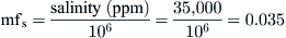
Saline water is a mixture of pure water and salt. A desalination plant performs a separation process in which the input saline water is separated into two output streams, those of brine and product water. The water produced from the process contains a low concentration of dissolved salts, whereas the brine contains the remaining high concentration of dissolved salts. Therefore, when analyzing desalination processes, the properties of salt and pure water must be taken into account. One of the most important properties in such analysis is salinity, usually expressed in parts per million (ppm), which is defined as: salinity = mass fraction (mfs) × 106. Therefore, a salinity of 2000 ppm corresponds to a salinity of 0.2%, or a salt mass fraction of mfs = 0.002. The mole fraction of salt, xs, is obtained from (Cengel et al., 1999):
Similarly,
![]() (8.2)
(8.2)
In Eqs (8.1) and (8.2), the subscripts s, w, and sw stand for salt, water, and saline water, respectively. The apparent molar mass of the saline water is (Cerci, 2002):
![]() (8.3)
(8.3)
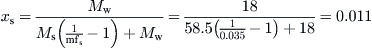
The molar mass of NaCl is 58.5 kg/kmol and the molar mass of water is 18.0 kg/kmol. Salinity is usually given in terms of mass fractions, but mole fractions are often required. Therefore, combining Eqs (8.1)–(8.3) and considering that xs + xw = 1 gives the following relations for converting mass fractions to mole fractions:
![]() (8.4)
(8.4)
and
![]() (8.5)
(8.5)
Solutions that have a concentration of less than 5% are considered to be dilute solutions, which closely approximate the behavior of an ideal solution, and thus the effect of dissimilar molecules on each other is negligible. Brackish underground water and even seawater are ideal solutions, since they have about a 4% salinity at most (Cerci, 2002).
EXAMPLE 8.1
Seawater of the Mediterranean Sea has a salinity of 35,000 ppm. Estimate the mole and mass fractions for salt and water.
Solution
From salinity, we get:
From Eq. (8.4), we get:
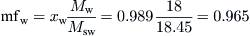
As xs + xw = 1, we have xw = 1 − xs = 1 − 0.011 = 0.989.
From Eq. (8.3),

Finally, from Eq. (8.2),
Extensive properties of a mixture are the sum of the extensive properties of its individual components. Thus, the enthalpy and entropy of a mixture are obtained from:
![]() (8.6)
(8.6)
and
![]() (8.7)
(8.7)
Dividing by the total mass of the mixture gives the specific quantities (per unit mass of mixture) as:
![]() (8.8)
(8.8)
and
![]() (8.9)
(8.9)
The enthalpy of mixing of an ideal gas mixture is zero because no heat is released or absorbed during mixing. Therefore, the enthalpy of the mixture and the enthalpies of its individual components do not change during mixing. Thus, the enthalpy of an ideal mixture at a specified temperature and pressure is the sum of the enthalpies of its individual components at the same temperature and pressure (Klotz and Rosenberg, 1994). This also applies for the saline solution.
The brackish or seawater used for desalination is at a temperature of about 15 °C (288.15 K), pressure of 1 atm (101.325 kPa), and a salinity of 35,000 ppm. These conditions can be taken to be the conditions of the environment (dead state in thermodynamics).
The properties of pure water are readily available in tabulated water and steam properties tables. Those of salt are calculated by using the thermodynamic relations for solids, which require the set of the reference state of salt to determine the values of properties at specified states. For this purpose, the reference state of salt is taken at 0 °C, and the values of enthalpy and entropy of salt are assigned a value of 0 at that state. Then the enthalpy and entropy of salt at temperature T can be determined from:
![]() (8.10)
(8.10)
![]() (8.11)
(8.11)
The specific heat of salt can be taken to be cps = 0.8368 kJ/kg K. The enthalpy and entropy of salt at To = 288.15 K can be determined to be hso = 12.552 kJ/kg and sso = 0.04473 kJ/kg K, respectively. It should be noted that, for incompressible substances, enthalpy and entropy are independent of pressure (Cerci, 2002).
EXAMPLE 8.2
Find the enthalpy and entropy of seawater at 40 °C.
Solution
From Eq. (8.10),

From Eq. (8.11),

Mixing is an irreversible process; hence, the entropy of a mixture at a specified temperature and pressure is greater than the sum of the entropies of the individual components at the same temperature and pressure before mixing. Therefore, since the entropy of a mixture is the sum of the entropies of its components, the entropies of the components of a mixture are greater than the entropies of the pure components at the same temperature and pressure. The entropy of a component per unit mole in an ideal solution at specified pressure P and temperature T is given by (Cengel and Boles, 1998):
![]() (8.12)
(8.12)
R = gas constant = 8.3145 kJ/kmol K.
It should be noted that ln(xi) is a negative quantity, as xi < 1, and therefore −R ln(xi) is always positive. Equation (8.12) proves the statement made earlier that the entropy of a component in a mixture is always greater than the entropy of that component when it exists alone at a temperature and pressure equal to that of the mixture. Finally, the entropy of a saline solution is the sum of the entropies of salt and water in the saline solutions (Cerci, 2002):
![]() (8.13)
(8.13)
The entropy of saline water per unit mass is determined by dividing the above quantity, which is per unit mole, by the molar mass of saline water. Therefore,
![]() (8.14)
(8.14)
The exergy of a flow stream is given as (Cengel and Boles, 1998):
![]() (8.15)
(8.15)
Finally, the rate of exergy flow associated with a fluid stream is given by:
![]() (8.16)
(8.16)
Using the relations presented in this section, the specific exergy and exergy flow rates at various points of a reverse osmosis system can be evaluated. From the exergy flow rates, the exergy destroyed within any component of the system can be determined from exergy balance. It should be noted that the exergy of raw brackish or seawater is 0, since its state is taken to be the dead state. Also, exergies of brine streams are negative because they have salinities above the dead state level.
8.2.2 Exergy analysis of thermal desalination systems
From the first law of thermodynamics, the energy balance equation can be obtained as:
![]() (8.17)
(8.17)
The mass, species, and energy balance equations for all the plant subsystems and a few associated state- and effect-related functions yield a set of independent equations. This set of simultaneous equations is solved by matrix algebra assuming equal temperature intervals for all effects and assuming that all effects have adiabatic walls. The boundary conditions are the specific seawater feed conditions (flow rate, salinity, temperature), the desired distillate production rate, and the specified maximum brine salinity and temperature. The matrix solutions obtained determine the distillation rates in the individual effects, the steam requirements, and hence the performance ratio (PR) (Hamed et al., 1996).
The steady-state exergy balance equation may be written as:

Therefore,
![]() (8.18)
(8.18)
where
![]() (8.19)
(8.19)
and
![]() (8.20)
(8.20)
The system overall irreversibility rate can be expressed as the summation of the subsystem irreversibility rate:
![]() (8.21)
(8.21)
where J is the number of subsystems in the analysis and Ii is the irreversibility rate of subsystem i. The exergy (or second law) efficiency ηII, given by:
![]() (8.22)
(8.22)
is used as a criterion of performance, with Ein and Eout determined by Eqs (8.19) and (8.20), respectively. The total loss of exergy is obtained from the individual exergy losses of the plant subsystems. The exergy efficiency defect, δi, of each subsystem is defined by (Hamed et al., 1996):
![]() (8.23)
(8.23)
Combining Eqs (8.22) and (8.23) gives:
![]() (8.24)
(8.24)
The exergy of the working fluid at each point, calculated from its properties, is given by:
![]() (8.25)
(8.25)
where the subscript o indicates the “dead state” or environment defined in the previous section.
Leave a Reply