Module design
Most commercial and industrial systems require a large number of collectors to satisfy the heating demand. Connecting the collectors with just one set of manifolds makes it difficult to ensure drainability and low pressure drop. It would also be difficult to balance the flow so as to have the same flow rate through all collectors. A module is a group of collectors that can be grouped into parallel flow and combined series–parallel flow. Parallel flow is more frequently used because it is inherently balanced, has a low pressure drop, and can be drained easily. Figure 5.20 illustrates the two most popular collector header designs: external and internal manifolds.
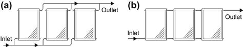
FIGURE 5.20 Collector manifolding arrangements for parallel flow modules. (a) External manifolding. (b) Internal manifolding.
Generally, flat-plate collectors are made to connect to the main pipes of the installation in one of the two methods shown in Figure 5.20. The external manifold collector has a small-diameter connection because it is used to carry the flow for only one collector. Therefore, each collector is connected individually to the manifold piping, which is not part of the collector panel. The internal manifold collector incorporates several collectors with large headers, which can be placed side by side to form a continuous supply and return manifold, so the manifold piping is integral with each collector. The number of collectors that can be connected depends on the size of the header.
External manifold collectors are generally more suitable for small systems. Internal manifolding is preferred for large systems because it offers a number of advantages. These are cost savings because the system avoids the use of extra pipes (and fittings), which need to be insulated and properly supported, and the elimination of heat losses associated with external manifolding, which increases the thermal performance of the system.
It should be noted that the flow is parallel but the collectors are connected in series. When arrays must be greater than one panel high, a combination of series and parallel flow may be used, as shown in Figure 5.21. This is a more suitable design in cases where collectors are installed on an inclined roof.
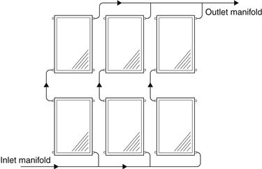
FIGURE 5.21 Collector manifolding arrangement for combined series-parallel flow modules.
The choice of series or parallel arrangement depends on the temperature required from the system. Connecting collectors in parallel means that all collectors have as input the same temperature, whereas when a series connection is used, the outlet temperature from one collector (or row of collectors) is the input to the next collector (or row of collectors). The performance of such an arrangement can be obtained from the equations presented in Chapter 4, Section 4.1.2.
5.4.2 Array design
An array usually includes many individual groups of collectors, called modules, to provide the necessary flow characteristics. To maintain a balanced flow, an array or field of collectors should be built from identical modules. Basically, two types of systems can be used: direct return and reverse return. In direct return, shown in Figure 5.22, balancing valves are needed to ensure uniform flow through the modules. The balancing valves must be connected at the module outlet to provide the flow resistance necessary to ensure filling of all modules on a pump start-up. Whenever possible, modules must be connected in a reverse-return mode, as shown in Figure 5.23. The reverse return ensures that the array is self-balanced, as all collectors operate with the same pressure drop: i.e., the first collector in the supply manifold is the last in the return manifold, the second on the supply side is the second before the last in the return, and so on. With proper design, an array can drain, which is an essential requirement for drain-back and drain-down freeze protection. For this to be possible, piping to and from the collectors must be sloped properly. Typically, piping and collectors must slope to drain with an inclination of 20 mm per linear meter (ASHRAE, 2004).
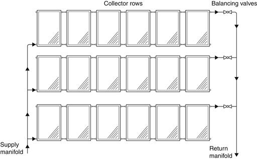
FIGURE 5.22 Direct-return array piping.
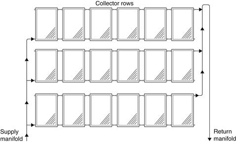
FIGURE 5.23 Reverse-return array piping.
External and internal manifold collectors have different mounting and plumbing considerations. A module with externally manifolded collectors can be mounted horizontally, as shown in Figure 5.24(a). In this case, the lower header must be pitched as shown. The slope of the upper header can be either horizontal or pitched toward the collectors, so it can drain through the collectors.
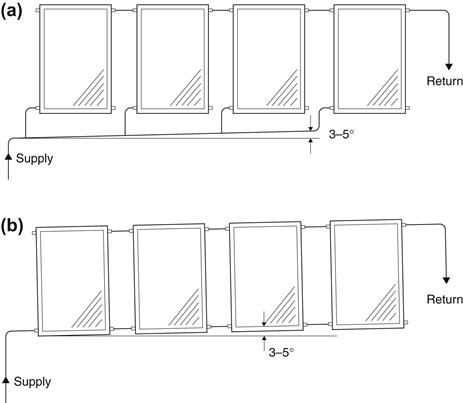
FIGURE 5.24 Mounting for drain-back collector modules. (a) External manifold. (b) Internal manifold.
Arrays with internal manifolds are a little more difficult to design and install. For these collectors to drain, the entire bank must be tilted, as shown in Figure 5.24(b). Reverse return always implies an extra pipe run, which is more difficult to drain, so sometimes in this case it is more convenient to use direct return.
Solar collectors should be oriented and sloped properly to maximize their performance. A collector in the Northern Hemisphere should be located to face due south and a collector in the Southern Hemisphere should face due north. The collectors should face as south or as north, depending on the case, as possible, although a deviation of up to 10° is acceptable. For this purpose, the use of a compass is highly recommended.
The optimum tilt angle for solar collectors depends on the longitude of the site. For maximum performance, the collector surface should be as perpendicular to the sun rays as possible. The optimum tilt can be calculated for each month of the year, but since a fixed inclination is used, an optimum slope throughout the year must be used. Some guidelines are given in Chapter 3, Section 3.1.1.
Shading
When large collector arrays are mounted on flat roofs or level ground, multiple rows of collectors are usually installed. These multiple rows should be spaced so they do not shade each other at low sun angles. For this purpose, the method presented in Chapter 2, Section 2.2.3, could be used. Figure 5.25 shows the shading situation. It can be shown that the ratio of the row spacing to collector height, b/a, for a south facing array is given by:
![]() (5.47a)
(5.47a)
A graphical solution of Eq. (5.47a) is shown in Figure 5.26, from which the b/a ratio can be read directly if the shading angle, θs, and collector inclination, β, are known. It should be noted that this is the shading that occurs at the meridian (12.00 noon), where solar azimuth angle, z, is zero. At any other time the shading distance bs, can be estimated using the solar azimuth angle, z, and solar altitude angle, α, from:
![]() (5.47b)
(5.47b)
Equations (5.47a) and (5.47b) neglect the thickness of the collector, which is small compared to dimensions a and b. If the piping, however, projects above the collector panels, it must be counted in the collector dimension a. The only unknown in Eq. (5.47a) is the shade angle, θs. To avoid shading completely, this can be found to be the minimum annual noon elevation, which occurs at noon on December 21. However, depending on the site latitude, this angle could produce very large row gaps (distance b), which might be not very practical. In this case, a compromise is usually made to allow some shading during winter months.
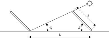
FIGURE 5.25 Row-to-row collector shading geometry.
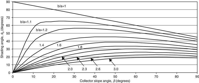
FIGURE 5.26 Graphic solution of collector row shading.
Thermal expansion
Another important parameter that needs to be considered is thermal expansion, which affects the modules of multi-collector array installations. Thermal expansion considerations deserve special attention in solar systems because of the temperature range within which the systems work. Thermal expansion (or contraction) of a module of collectors in parallel may be estimated by the following (ASHRAE, 2004):
![]() (5.48)
(5.48)
Δ = expansion or contraction of the collector array (mm);
n = number of collectors in the array;
tmax = collector stagnation temperature (°C), see Chapter 4, Eq. (4.7); and
ti = temperature of the collector when installed (°C).
Expansion considerations are very important, especially in the case of internal collector manifolds. These collectors should have a floating absorber plate, i.e., the absorber manifold should not be fastened to the collector casing, so it can move freely by a few millimeters within the case.
Galvanic corrosion
Galvanic corrosion is caused by the electrical contact between dissimilar metals in a fluid stream. It is therefore very important not to use different materials for the collector construction and piping manifolds. For example, if copper is used for the construction of the collector, the supply and return piping should also be made from copper. Where different metals must be used, dielectric unions between dissimilar metals must be used to prevent electrical contact. Of the possible metals used to construct collectors, aluminum is the most sensitive to galvanic corrosion, because of its position in the galvanic series. This series, shown in Table 5.5, indicates the relative activity of one metal against another. Metals closer to the anodic end of the series tend to corrode when placed in electrical contact with another metal that is closer to the cathodic end of the series in a solution that conducts electricity, such as water.
Table 5.5
Galvanic Series of Common Metals and Alloys
Corroded End (Anodic)
Magnesium
Zinc
Aluminum
Carbon steel
Brass
Tin
Copper
Bronze
Stainless steel
Protected End (Cathodic)
Array sizing
The size of a collector array depends on the cost, available roof or ground area, and percent of the thermal load required to be covered by the solar system. The first two parameters are straightforward and can easily be determined. The last, however, needs detailed calculations, which take into consideration the available radiation, performance characteristics of the chosen collectors, and other, less important parameters. For this purpose, methods and techniques that will be covered in other chapters of this book can be used, such as the f-chart method, utilizability method, and the use of computer simulation programs (see Chapter 11).
It should be noted that, because the loads fluctuate on a seasonal basis, it is not cost-effective to have the solar system provide all the required energy, because if the array is sized to handle the months with the maximum load it will be oversized for the months with minimum load.
Heat exchangers
The function of a heat exchanger is to transfer heat from one fluid to another. In solar applications, usually one of the two fluids is the domestic water to be heated. In closed solar systems, it also isolates circuits operating at different pressures and separates fluids that should not be mixed. As was seen in the previous section, heat exchangers for solar applications may be placed either inside or outside the storage tank. The selection of a heat exchanger involves considerations of performance (with respect to heat exchange area), guaranteed fluid separation (double-wall construction), suitable heat exchanger material to avoid galvanic corrosion, physical size and configuration (which may be a serious problem in internal heat exchangers), pressure drop caused (influence energy consumption), and serviceability (providing access for cleaning and scale removal).
External heat exchangers should also be protected from freezing. The factors that should be considered when selecting an external heat exchanger for a system protected by a non-freezing fluid that is exposed to extreme cold are the possibility of freeze-up of the water side of the heat exchanger and the performance loss due to extraction of heat from storage to heat the low-temperature fluid.
The combination of a solar collector and a heat exchanger performs exactly like a collector alone with a reduced FR. The useful energy gain from a solar collector is given by Eq. (4.3). The collector heat exchanger arrangement is shown in Figure 5.27. Therefore, Eqs (4.2) and (4.3), with the symbol convention shown in Figure 5.27, can be written as:
![]() (5.49a)
(5.49a)
![]() (5.49b)
(5.49b)
The plus sign indicates that only positive values should be considered.
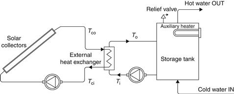
FIGURE 5.27 Schematic diagram of a liquid system with an external heat exchanger between the solar collectors and storage tank.
In addition to size and surface area, the configuration of the heat exchanger is important for achieving maximum performance. The heat exchanger performance is expressed in terms of its effectiveness. By neglecting any piping losses, the collector energy gain transferred to the storage fluid across the heat exchanger is given by:
![]() (5.50)
(5.50)
![]() = smaller of the fluid capacitance rates of the collector and tank sides of the heat exchanger (W/°C);
= smaller of the fluid capacitance rates of the collector and tank sides of the heat exchanger (W/°C);
Tco = hot (collector loop) stream inlet temperature (°C); and
Ti = cold (storage) stream inlet temperature (°C).
The effectiveness, ε, is the ratio between the heat actually transferred and the maximum heat that could be transferred for a given flow and fluid inlet temperature conditions. The effectiveness is relatively insensitive to temperature, but it is a strong function of a heat exchanger design. A designer must decide what heat exchanger effectiveness is required for the specific application. The effectiveness for a counterflow heat exchanger is given by the following:
If C ≠ 1
If C = 1,
![]() (5.52)
(5.52)
where NTU = number of transfer units given by:
![]() (5.53)
(5.53)
And the dimensionless capacitance rate, C, is given by:
![]() (5.54)
(5.54)
For heat exchangers located in the collector loop, the minimum flow usually occurs on the collector side rather than the tank side.
Solving Eq. (5.49a) for Tci and substituting into Eq. (5.49b) gives:
![]() (5.55)
(5.55)
Solving Eq. (5.50) for Tco and substituting into Eq. (5.55) gives:
![]() (5.56)
(5.56)
In Eq. (5.56), the modified collector heat removal factor takes into account the presence of the heat exchanger and is given by:
![]() (5.57)
(5.57)
In fact, the factor ![]() is the consequence, on the collector performance, that occurs because the heat exchanger causes the collector side of the system to operate at a higher temperature than a similar system without a heat exchanger. This can also be viewed as the increase of collector area required to have the same performance as a system without a heat exchanger.
is the consequence, on the collector performance, that occurs because the heat exchanger causes the collector side of the system to operate at a higher temperature than a similar system without a heat exchanger. This can also be viewed as the increase of collector area required to have the same performance as a system without a heat exchanger.
EXAMPLE 5.4
A counterflow heat exchanger is located between a collector and a storage tank. The fluid in the collector side is a water–glycol mixture with cp = 3840 J/kg °C and a flow rate of 1.35 kg/s, whereas the fluid in the tank side is water with a flow rate of 0.95 kg/s. If the UA of the heat exchanger is 5650 W/°C, the hot glycol enters the heat exchanger at 59 °C, and the water from the tank at 39 °C, estimate the heat exchange rate.
Solution
First, the capacitance rates for the collector and tank sides are required, given by:


From Eq. (5.54), the heat exchanger dimensionless capacitance rate is equal to:
From Eq. (5.53),
From Eq. (5.51),
Finally, from Eq. (5.50),

EXAMPLE 5.5
Redo the preceding example; if FRUL = 5.71 W/m2 °C and collector area is 16 m2, what is the ratio ![]() ?
?
Solution
All data are available from the previous example. So, from Eq. (5.57),

This result indicates that 2% more collector area would be required for the system with a heat exchanger to deliver the same amount of solar energy as a similar system without a heat exchanger.
Pipe and duct losses
The collector performance equation can be modified to include the heat losses from the collector loop piping. The analysis is done by considering that there is a temperature drop ΔTi from the outlet of the storage tank to the inlet of the collector (Beckman, 1978). Thus, the temperature inlet to the collector is Ti − ΔTi and Eq. (3.60) becomes:
![]() (5.58)
(5.58)
The pipe losses can be obtained from the following integral for both the inlet and outlet portions:
![]() (5.59)
(5.59)
Up = the loss coefficient from the pipe (W/m2 K)
Equation (5.59) can be integrated but as pipes are usually well insulated the losses are very small and the integral can be approximated with good accuracy in terms of the collector inlet and outlet temperatures by:
![]() (5.60)
(5.60)
Estimating To from the right part of Eq. (3.31) and applying in Eq. (5.60), gives:
![]() (5.61)
(5.61)
The temperature decrease, ΔTi, due to the heat losses from storage tank to the inlet of the collector can be obtained with satisfactory accuracy from (Beckman, 1978):
![]() (5.62)
(5.62)
Substituting Eqs (5.61) and (5.62) into Eq. (5.58) and performing various manipulations, the rate of useful energy gain by considering the collector and its piping is given by:
 (5.63)
Equation (5.63) can be written in the same way as Eq. (3.60) by using modified values of (τα)′ and UL′ as:
![]() (5.64a)
(5.64a)
![]() (5.64b)
(5.64b)
and
 (5.64c)
It should be noted that the same analysis can be applied to air collectors with respect to supply and return ducts and in this case the appropriate symbols are used for duct instead of pipe, i.e., Ud in place of Up, Ad,i in place of Ap,i and Ad,o in place of Ap,o.
Partially shaded collectors
In some cases, shading is either unavoidable or can be accepted in a few days during winter, especially for solar cooling applications, where the maximum requirement is during summer and shading effects are minimal due to the high sun altitude angle. Shading usually occurs at the bottom part of the collector in the second and subsequent rows of an array. The shaded part receives only diffuse radiation whereas the non-shaded part receives both direct and diffuse radiations. When shading occurs, the performance of the collectors can be estimated by considering an average value of radiation over the whole collector area or by considering the detailed analysis presented here. This situation is presented in Figure 5.28 where as indicated the two parts of the collector receive radiation Gt1 and Gt2. The temperature entering the first part of area A1 is Ti and the temperature entering the second part of area A2 is To,1, i.e., the hypothetical output of part 1. As the collector is “one unit” the values of FR and UL are the same for the two parts, whereas as the angle of incidence in the two parts are different (bottom part receives only diffuse radiation from the sky dome it sees) the (τα) product for the two parts will be different. Applying Eq. (3.60) for the two parts we get:
![]() (5.65)
(5.65)
![]() (5.66)
(5.66)
The rate of useful energy from the bottom part is equal to:
![]() (5.67)
(5.67)
![]() (5.68)
(5.68)
By applying Eq. (5.68) into Eq. (5.66) to eliminate To,1, and adding Eqs (5.65) and (5.66), to get the total rate useful energy gain from the whole collector, we obtain:
![]() (5.69)
(5.69)
where,
![]() (5.70)
(5.70)
In calculations and as the position of the sun in the sky changes continuously, the two areas A1 and A2 will be functions of time.
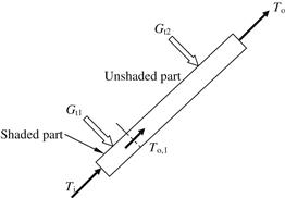
FIGURE 5.28 Partly shaded solar collector.
Over-temperature protection
Periods of high insolation and low load result in overheating of the solar energy system. Overheating can cause liquid expansion or excessive pressure, which may burst piping or storage tanks. Additionally, systems that use glycols are more problematic, since glycols break down and become corrosive at temperatures greater than 115 °C. Therefore, the system requires protection against this condition. The solar system can be protected from overheating by a number of methods, such as:
• Stopping circulation in the collection loop until the storage temperature decreases (in air systems);
• Discharging the overheated water from the system and replacing it with cold make-up water; and
• Using a heat exchanger coil for rejecting heat to the ambient air.
As will be seen in the next section, controllers are available that can sense over-temperature. The normal action taken by such a controller is to turn off the solar pump to stop heat collection. In a drain-back system, after the solar collectors are drained, they attain stagnation temperatures; therefore, the collectors used for these systems should be designed and tested to withstand over-temperature. In addition, drain-back panels should withstand the thermal shock of start-up when relatively cool water enters the solar collectors while they are at stagnation temperature.
In a closed loop antifreeze system that has a heat exchanger, if circulation stops, high stagnation temperatures occur. As indicated previously, these temperatures could break down the glycol heat transfer fluid. To prevent damage of equipment or injury due to excessive pressure, a pressure relief valve must be installed in the loop, as indicated in the various system diagrams presented earlier in this chapter, and a means of rejecting heat from the collector loop must be provided. The pressure relief valve should be set to relieve below the operating pressure of the component with the smallest operating pressure in the closed loop system.
It should be noted that, when the pressure relief valve is open, it discharges expensive antifreeze solution, which may damage roof membranes. Therefore, the discharge can be piped to containers to save antifreeze, but the designer of such a system must pay special attention to safety issues because of the high pressures and temperatures involved.
Another point that should be considered is that, if a collector loop containing glycol stagnates, chemical decomposition raises the fusion point of the liquid and the fluid would not be able to protect the system from freezing.
The last option indicated previously is the use of a heat exchanger that dumps heat to the ambient air or other sink. In this system, fluid circulation continues, but this is diverted from storage through a liquid-to-air heat exchanger, as shown in Figure 5.29. For this system, a sensor is used on the solar collector absorber plate that turns on the heat rejection equipment. When the sensor reaches the high-temperature set point, it turns on the pump and the fan. These continue to operate until the over-temperature controller senses that the temperature is within the safety limits and resets the system to its normal operating state.
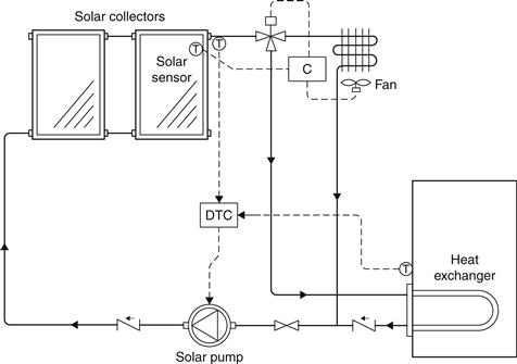
FIGURE 5.29 Heat rejection by a solar heating system using a liquid-to-air heat exchanger.
Leave a Reply