
In this section, the thermal analysis of the collectors is presented. The two major types of collectors, flat plate and concentrating, are examined separately. The basic parameter to consider is the collector thermal efficiency. This is defined as the ratio of the useful energy delivered to the energy incident on the collector aperture. The incident solar flux consists of direct and diffuse radiation. While flat-plate collectors can collect both, concentrating collectors can utilize direct radiation only if the concentration ratio is greater than 10 (Prapas et al., 1987).
In this section, the various relations required to determine the useful energy collected and the interaction of the various constructional parameters on the performance of a collector are presented.
3.3.1 Absorbed solar radiation
The prediction of collector performance requires information on the solar energy absorbed by the collector absorber plate. The solar energy incident on a tilted surface can be found by the methods presented in Chapter 2. As can be seen from Chapter 2, the incident radiation has three special components: beam, diffuse, and ground-reflected radiation. This calculation depends on the radiation model employed. Using the isotropic model on an hourly basis, Eq. (2.97) can be modified to give the absorbed radiation, S, by multiplying each term with the appropriate transmittance–absorptance product as follows:
![]() (3.1a)
(3.1a)
where the terms [1 + cos(β)]/2 and [1 − cos(β)]/2 are the view factors from the collector to the sky and from the collector to the ground, respectively. The same equation can be used to estimate the monthly average absorbed solar radiation, ![]() by replacing the hourly direct and diffuse radiation values with the appropriate monthly average values,
by replacing the hourly direct and diffuse radiation values with the appropriate monthly average values, ![]() and
and ![]() , RB with
, RB with ![]() , and various (τα) values with monthly average values,
, and various (τα) values with monthly average values,![]() in Eq. (3.1a):
in Eq. (3.1a):
![]() (3.1b)
(3.1b)
More details on this are given in Chapter 11.
The combination of cover with the absorber plate is shown in Figure 3.26, together with a ray tracing of the radiation. As can be seen, of the incident energy falling on the collector, τα is absorbed by the absorber plate and (1 − α)τ is reflected back to the glass cover. The reflection from the absorber plate is assumed to be diffuse, so the fraction (1 − α)τ that strikes the glass cover is diffuse radiation and (1 − α)τρD is reflected back to the absorber plate. The multiple reflection of diffuse radiation continues so that the fraction of the incident solar energy ultimately absorbed is:
![]() (3.2)
(3.2)
Typical values of (τα) are 0.7–0.75 for window glass and 0.85–0.9 for low-iron glass. A reasonable approximation of Eq. (3.2) for most practical solar collectors is:
![]() (3.3)
(3.3)
The reflectance of the glass cover for diffuse radiation incident from the absorber plate, ρD, can be estimated from Eq. (2.57) as the difference between τα and τ at an angle of 60°. For single covers, the following values can be used for ρD:
For a given collector tilt angle, β, the following empirical relations, derived by Brandemuehl and Beckman (1980), can be used to find the effective incidence angle for diffuse radiation from sky, θe,D, and ground-reflected radiation, θe,G:
![]() (3.4a)
(3.4a)
![]() (3.4b)
(3.4b)
β = collector slope angle in degrees.
The proper transmittance can then be obtained from Eq. (2.53), whereas the angle-dependent absorptance from 0° to 80° can be obtained from Beckman et al. (1977):
![]() (3.5a)
(3.5a)
or from the polynomial fit for 0° to 90° from (Duffie and Beckman, 2006):
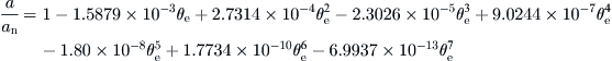 (3.5b)
θe = effective incidence angle (degrees).
an = absorptance at normal incident angle, which can be found from the properties of the absorber.
Subsequently, Eq. (3.2) can be used to find (τα)D and (τα)G. The incidence angle, θ, of the beam radiation required to estimate RB can be used to find (τα)B.
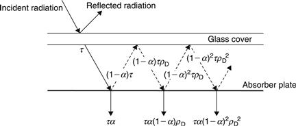
FIGURE 3.26 Radiation transfer between the glass cover and absorber plate.
Alternatively, (τα)n can be found from the properties of the cover and absorber materials, and Figure 3.27 can be used at the appropriate angle of incidence for each radiation component to find the three transmittance–absorptance products.
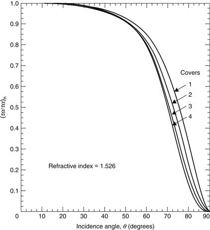
FIGURE 3.27 Typical (τα)/(τα)n curves for one to four glass covers. Reprinted from Klein (1979), with permission from Elsevier.
When measurements of incident solar radiation (It) are available, instead of Eq. (3.1a), the following relation can be used:
![]() (3.6)
(3.6)
where (τα)av can be obtained from:
EXAMPLE 3.1
For a clear winter day, IB = 1.42 MJ/m2 and ID = 0.39 MJ/m2. Ground reflectance is 0.5, incidence angle is 23°, and RB = 2.21. Calculate the absorbed solar radiation by a collector having a glass with KL = 0.037, the absorptance of the plate at normal incidence, an = 0.91, and the refraction index of glass is 1.526. The collector slope is 60°.
Solution
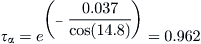
Using Eq. (3.5a) for the beam radiation at θ = 23°,
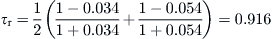
For the transmittance we need to calculate τα and τr. For the former, Eq. (2.51) can be used. From Eq. (2.44), θ2 = 14.8°. Therefore,
From Eqs (2.45) and (2.46) ![]() and
and ![]() . Therefore, from Eq. (2.50a),
. Therefore, from Eq. (2.50a),
Finally, from Eq. (2.53),

Alternatively, Eq. (2.52a) could be used with the above r values to obtain τ directly.
From Eq. (3.3),

From Eq. (3.4a), the effective incidence angle for diffuse radiation is:

From Eq. (3.5a), for the diffuse radiation at θ = 57°, a/an = 0.949.
From Eq. (2.44), for θ1 = 57°, θ2 = 33°. From Eqs (2.45) and (2.46), ![]() and
and ![]()
From Eq. (2.50a), τr = 0.858, and from Eq. (2.51), τα = 0.957. From Eq. (2.53),

and from Eq. (3.3),

From Eq. (3.4b), the effective incidence angle for ground-reflected radiation is:

From Eq. (3.5a), for the ground-reflected radiation at θ = 65°, a/an = 0.897.
From Eq. (2.44), for θ1 = 65°, θ2 = 36°. From Eqs (2.45) and (2.46), ![]() and
and ![]()
From Eq. (2.50a), τr = 0.792, and from Eq. (2.51), τα = 0.955. From Eq. (2.53),

And from Eq. (3.3),

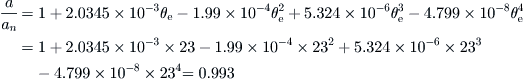
In a different way, from Eq. (3.3),
(τα)n = 1.01 × 0.884 × 0.91 = 0.812 (note that for the transmittance the value for normal incidence is used, i.e., τn).
From Figure 3.27, for beam radiation at θ = 23°, (τα)/(τα)n = 0.98. Therefore,

From Figure 3.27, for diffuse radiation at θ = 57°, (τα)/(τα)n = 0.89. Therefore,

From Figure 3.27, for ground-reflected radiation at θ = 65°, (τα)/(τα)n = 0.76. Therefore,

All these values are very similar to the previously found values, but the effort required is much less.
Finally, the absorbed solar radiation is obtained from Eq. (3.1a):

3.3.2 Collector energy losses
When a certain amount of solar radiation falls on the surface of a collector, most of it is absorbed and delivered to the transport fluid, and it is carried away as useful energy. However, as in all thermal systems, heat losses to the environment by various modes of heat transfer are inevitable. The thermal network for a single-cover FPC in terms of conduction, convection, and radiation is shown in Figure 3.28(a) and in terms of the resistance between plates in Figure 3.28(b). The temperature of the plate is Tp, the collector back temperature is Tb, and the absorbed solar radiation is S. In a simplified way, the various thermal losses from the collector can be combined into a simple resistance, RL, as shown in Figure 3.28(c), so that the energy losses from the collector can be written as:
![]() (3.8)
(3.8)
UL = overall heat loss coefficient based on collector area Ac (W/m2 K).
The overall heat loss coefficient is a complicated function of the collector construction and its operating conditions, given by the following expression:
![]() (3.9)
(3.9)
Ut = top loss coefficient (W/m2 K).
Ub = bottom heat loss coefficient (W/m2 K).
Ue = heat loss coefficient from the collector edges (W/m2 K).
Therefore, UL is the heat transfer resistance from the absorber plate to the ambient air. All these coefficients are examined separately. It should be noted that edge losses are not shown in Figure 3.28.
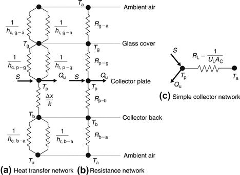
FIGURE 3.28 Thermal network for a single-cover collector in terms of (a) conduction, convection, and radiation; (b) resistance between plates; and (c) a simple collector network.
In addition to serving as a heat trap by admitting shortwave solar radiation and retaining longwave thermal radiation, the glazing also reduces heat loss by convection. The insulating effect of the glazing is enhanced by the use of several sheets of glass or glass plus plastic.
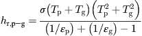
Under steady-state conditions, the heat transfer from the absorber plate to the glass cover is the same as the energy lost from the glass cover to ambient. As shown in Figure 3.28, the heat transfer upward from the absorber plate at temperature Tp to the glass cover at Tg and from the glass cover at Tg to ambient at Ta is by convection and infrared radiation. For the infrared radiation heat loss, Eq. (2.67) can be used. Therefore, the heat loss from absorber plate to glass is given by:
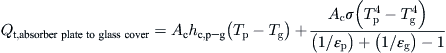 (3.10)
hc,p–g = convection heat transfer coefficient between the absorber plate and glass cover (W/m2 K).
εp = infrared emissivity of absorber plate.
εg = infrared emissivity of glass cover.
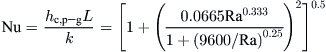
For tilt angles up to 60°, the convective heat transfer coefficient, hc,p–g, is given by Hollands et al. (1976) for collector inclination (β) in degrees:
![]() (3.11)
(3.11)
where the plus sign represents positive values only. The Rayleigh value, Ra, is given by:
![]() (3.12)
(3.12)
g = gravitational constant, = 9.81 m2/s.
β′ = volumetric coefficient of expansion; for ideal gas, β′ = 1/T.
L = absorber to glass cover distance (m).
The fluid properties in Eq. (3.12) are evaluated at the mean gap temperature (Tp + Tg)/2.
For vertical collectors, the convection correlation is given by Shewen et al. (1996) as:
 (3.13)
The radiation term in Eq. (3.10) can be linearized by the use of Eq. (2.73) as:
 (3.14)
Consequently, Eq. (3.10) becomes:
![]() (3.15)
(3.15)
in which:
Similarly, the heat loss from glass cover to ambient is by convection to the ambient air (Ta) and radiation exchange with the sky (Tsky). For convenience, the combined convection–radiation heat transfer is usually given in terms of Ta only by:
![]() (3.17)
(3.17)
hc,g–a = convection heat transfer coefficient between the glass cover and ambient due to wind (W/m2 K).
hr,g–a = radiation heat transfer coefficient between the glass cover and ambient (W/m2 K).
The radiation heat transfer coefficient is now given by Eq. (2.75), noting that, instead of Tsky, Ta is used for convenience, since the sky temperature does not affect the results much:
![]() (3.18a)
(3.18a)
If the sky temperature is considered:
![]() (3.18b)
(3.18b)
The atmosphere does not have a uniform temperature. It radiates selectively at certain wavelengths and is essentially transparent in the wavelength range from 8 to 14 μm, while outside this range has absorbing bands covering much of the far infrared spectrum. Several relations have been proposed to associate Tsky (K) with measured meteorological variables. Two of them are given here:
Swinbank (1963) correlation:
![]() (3.18c)
(3.18c)
Berdahl and Martin (1984) correction:
![]() (3.18d)
(3.18d)
Tdp = dew point temperature (°C)
From Eq. (3.17),
![]() (3.19)
(3.19)
Since resistances Rp–g and Rg–a are in series, their resultant is given by:
Therefore,
![]() (3.21)
(3.21)
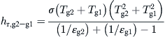
In some cases, collectors are constructed with two glass covers in an attempt to lower heat losses. In this case, another resistance is added to the system shown in Figure 3.28 to account for the heat transfer from the lower to the upper glass covers. By following a similar analysis, the heat transfer from the lower glass at Tg2 to the upper glass at Tg1 is given by:
![]() (3.22)
(3.22)
hc,g2–g1 = convection heat transfer coefficient between the two glass covers (W/m2 K).
hr,g2–g1 = radiation heat transfer coefficient between the two glass covers (W/m2 K).
The convection heat transfer coefficient can be obtained by Eqs (3.11–3.13). The radiation heat transfer coefficient can be obtained again from Eq. (2.73) and is given by:
 (3.23)
where εg2 and εg1 are the infrared emissivities of the top and bottom glass covers.
Finally, the resistance Rg2–g1 is given by:
![]() (3.24)
(3.24)
In the case of collectors with two covers, Eq. (3.24) is added on the resistance values in Eq. (3.20). The analysis of a two-cover collector is given in Example 3.2.
In the preceding equations, solutions by iterations are required for the calculation of the top heat loss coefficient, Ut, since the air properties are functions of operating temperature. Because the iterations required are tedious and time consuming, especially for the case of multiple-cover systems, straightforward evaluation of Ut is given by the following empirical equation with sufficient accuracy for design purposes (Klein, 1975):
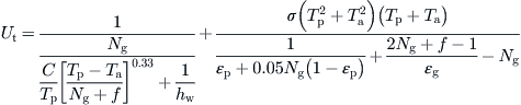 (3.25)
where
![]() (3.27)
(3.27)
![]() (3.28)
(3.28)
It should be noted that, for the wind heat transfer coefficient, no well-established research has been undertaken yet, but until this is done, Eq. (3.28) can be used. The minimum value of hw for still air conditions is 5 W/m2 °C. Therefore, if Eq. (3.28) gives a lower value, this should be used as a minimum.
The energy loss from the bottom of the collector is first conducted through the insulation and then by a combined convection and infrared radiation transfer to the surrounding ambient air. Because the temperature of the bottom part of the casing is low, the radiation term (hr,b–a) can be neglected; thus the energy loss is given by:
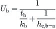 (3.29)
tb = thickness of back insulation (m).
kb = conductivity of back insulation (W/m K).
hc,b–a = convection heat loss coefficient from back to ambient (W/m2 K).
The conduction resistance of the insulation behind the collector plate governs the heat loss from the collector plate through the back of the collector casing. The heat loss from the back of the plate rarely exceeds 10% of the upward loss. Typical values of the back surface heat loss coefficient are 0.3–0.6 W/m2 K.
In a similar way, the heat transfer coefficient for the heat loss from the collector edges can be obtained from:
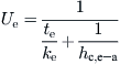 (3.30)
te = thickness of edge insulation (m).
ke = conductivity of edge insulation (W/m K).
hc,e–a = convection heat loss coefficient from edge to ambient (W/m2 K).
As the UL in Eq. (3.8) is multiplied by Ac the heat loss coefficient from the collector edges must be multiplied by Ae/Ac, where Ae is the total area of the four edges of the collector. The same applies for the bottom heat loss coefficient which must be multiplied by Ab/Ac if the two areas are not the same.
Typical values of the edge heat loss coefficient are 1.5–2.0 W/m2 K.
EXAMPLE 3.2
Estimate the top heat loss coefficient of a collector that has the following specifications:
Collector area = 2 m2 (1 × 2 m).
Thickness of each glass cover = 4 mm.
Thickness of absorbing plate = 0.5 mm.
Space between glass covers = 20 mm.
Space between inner glass cover and absorber = 40 mm.
Mean absorber temperature, Tp = 80 °C = 353 K.
Ambient air temperature = 15 °C = 288 K.
Absorber plate emissivity, εp = 0.10.
Solution
To solve this problem, the two glass cover temperatures are guessed and then by iteration are corrected until a satisfactory solution is reached by satisfying the following equations, obtained by combining Eqs (3.15), (3.17), and (3.22):

However, to save time in this example, close to correct values are used. Assuming that Tg1 = 23.8 °C (296.8 K) and Tg2 = 41.7 °C (314.7 K), from Eq. (3.14),

Similarly, for the two covers, we have:

From Eq. (3.18a) and noting that as no data are given Tsky = Ta, we have:

From Table A5.1, in Appendix 5, the following properties of air can be obtained:
For ½(Tp + Tg2) = ½(353 + 314.7) = 333.85 K,

For ½(Tg2 + Tg1) = ½(314.7 + 296.8) = 305.75 K,

By using these properties, the Rayleigh number, Ra, can be obtained from Eq. (3.12) and by noting that β′ = 1/T.
For hc,p–g2,

For hc,g2–g1,

Therefore, from Eq. (3.11), we have the following.
For hc,p–g2,
For hc,g2–g1,

The convection heat transfer coefficient from glass to ambient is the wind loss coefficient given by Eq. (3.28). In this equation, the characteristic length is the length of the collector, equal to 2 m.
Therefore,

To check whether the assumed values of Tg1 and Tg2 are correct, the heat transfer coefficients are substituted into Eqs (3.15), (3.17), and (3.22):


Since these three answers are not exactly equal, further trials should be made by assuming different values for Tg1 and Tg2. This is a laborious process which, however, can be made easier by the use of a computer and artificial intelligence techniques, such as a genetic algorithm (see Chapter 11). Following these techniques, the values that solve the problem are Tg1 = 296.80 K and Tg2 = 314.81 K. These two values give Qt/Ac = 143.3 W/m2 for all cases. If we assume that the values Tg1 = 296.8 K and Tg2 = 314.7 K are correct (remember, they were chosen to be almost correct from the beginning), Ut can be calculated from:

EXAMPLE 3.3
Repeat Example 3.2 using the empirical Eq. (3.25) and compare the results.
Solution
First, the constant parameters are estimated. The value of hw is already estimated in Example 3.2 and is equal to 11.294 W/m2 K.
From Eq. (3.26),


From Eq. (3.27),


Therefore, from Eq. (3.25),

The difference between this value and the one obtained in Example 3.2 is only 4.6%, but the latter was obtained with much less effort.
3.3.3 Temperature distribution between the tubes and collector efficiency factor
Under steady-state conditions, the rate of useful heat delivered by a solar collector is equal to the rate of energy absorbed by the heat transfer fluid minus the direct or indirect heat losses from the surface to the surroundings (see Figure 3.29). As shown in Figure 3.29, the absorbed solar radiation is equal to Gt(τα), which is similar to Eq. (3.6). The thermal energy lost from the collector to the surroundings by conduction, convection, and infrared radiation is represented by the product of the overall heat loss coefficient, UL, times the difference between the plate temperature, Tp, and the ambient temperature, Ta. Therefore, in a steady state, the rate of useful energy collected from a collector of area Ac can be obtained from:
![]() (3.31)
(3.31)
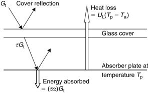
FIGURE 3.29 Radiation input and heat loss from a flat-plate collector.
Equation (3.31) can also be used to give the amount of useful energy delivered in joules (not rate in watts), if the irradiance Gt (W/m2) is replaced with irradiation It (J/m2) and we multiply UL, which is given in watts per square meter-degrees Centigrade (W/m2 °C), by 3600 to convert to joules per square meter-degrees Centigrade (J/m2 °C) for estimations with step of 1 h.
To model the collector shown in Figure 3.29, a number of assumptions, which simplify the problem, need to be made. These assumptions are not against the basic physical principles and are as follows:
1. The collector is in a steady state.
2. The collector is of the header and riser type fixed on a sheet with parallel tubes.
3. The headers cover only a small area of the collector and can be neglected.
4. Heaters provide uniform flow to the riser tubes.
5. Flow through the back insulation is one dimensional.
6. The sky is considered as a blackbody for the long-wavelength radiation at an equivalent sky temperature. Since the sky temperature does not affect the results much, this is considered equal to the ambient temperature.
7. Temperature gradients around tubes are neglected.
8. Properties of materials are independent of temperature.
9. No solar energy is absorbed by the cover.
10. Heat flow through the cover is one dimensional.
11. Temperature drop through the cover is negligible.
12. Covers are opaque to infrared radiation.
13. Same ambient temperature exists at the front and back of the collector.
14. Dust effects on the cover are negligible.
15. There is no shading of the absorber plate.
The collector efficiency factor can be calculated by considering the temperature distribution between two pipes of the collector absorber and assuming that the temperature gradient in the flow direction is negligible (Duffie and Beckman, 2006). This analysis can be performed by considering the sheet–tube configuration shown in Figure 3.30(a), where the distance between the tubes is W, the tube diameter is D, and the sheet thickness is δ. Since the sheet metal is usually made from copper or aluminum, which are good conductors of heat, the temperature gradient through the sheet is negligible; therefore, the region between the center line separating the tubes and the tube base can be considered as a classical fin problem.
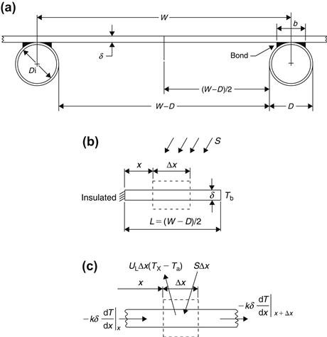
FIGURE 3.30 Flat-plate sheet and tube configuration. (a) Schematic diagram. (b) Energy balance for the fin element. (c) Energy balance for the tube element.
The fin, shown in Figure 3.30(b), is of length L = (W − D)/2. An elemental region of width, Δx, and unit length in the flow direction are shown in Figure 3.30(c). The solar energy absorbed by this small element is SΔx and the heat loss from the element is ULΔx(Tx − Ta), where Tx is the local plate temperature. Therefore, an energy balance on this element gives:
![]() (3.32)
(3.32)
where S is the absorbed solar energy. Dividing through with Δx and finding the limit as Δx approaches 0 gives:
The two boundary conditions necessary to solve this second-order differential equation are:

and

For convenience, the following two variables are defined:
![]() (3.34)
(3.34)
![]() (3.35)
(3.35)
Therefore, Eq. (3.33) becomes:
![]() (3.36)
(3.36)
which has the boundary conditions:

and
Equation (3.36) is a second-order homogeneous linear differential equation whose general solution is:
![]() (3.37)
(3.37)
The first boundary yields C1 = 0, and the second boundary condition yields:
or
With C1 and C2 known, Eq. (3.37) becomes:
![]() (3.38)
(3.38)
This equation gives the temperature distribution in the x direction at any given y.
The energy conducted to the region of the tube per unit length in the flow direction can be found by evaluating the Fourier’s law at the fin base (Kalogirou, 2004):
![]() (3.39)
(3.39)
However, kδm/UL is just 1/m. Equation (3.39) accounts for the energy collected on only one side of the tube; for both sides, the energy collection is:
![]() (3.40)
(3.40)
or with the help of fin efficiency,
![]() (3.41)
(3.41)
where factor F in Eq. (3.41) is the standard fin efficiency for straight fins with a rectangular profile, obtained from:
![]() (3.42)
(3.42)
The useful gain of the collector also includes the energy collected above the tube region. This is given by:
![]() (3.43)
(3.43)
Accordingly, the useful energy gain per unit length in the direction of the fluid flow is:
![]() (3.44)
(3.44)
This energy ultimately must be transferred to the fluid, which can be expressed in terms of two resistances as:
![]() (3.45)
(3.45)
where hfi = heat transfer coefficient between the fluid and the tube wall (see Section 3.6.4 for details).
In Eq. (3.45), Cb is the bond conductance, which can be estimated from knowledge of the bond thermal conductivity, kb, the average bond thickness, γ, and the bond width, b. The bond conductance on a per unit length basis is given by (Kalogirou, 2004):
![]() (3.46)
(3.46)
The bond conductance can be very important in accurately describing the collector performance. Generally it is necessary to have good metal-to-metal contact so that the bond conductance is greater than 30 W/m K, and preferably the tube should be welded to the fin.
Solving Eq. (3.45) for Tb, substituting it into Eq. (3.44), and solving the resultant equation for the useful gain, we get:
![]() (3.47)
(3.47)
where F′ is the collector efficiency factor, given by:
 (3.48)
A physical interpretation of F′ is that it represents the ratio of the actual useful energy gain to the useful energy gain that would result if the collector-absorbing surface had been at the local fluid temperature. It should be noted that the denominator of Eq. (3.48) is the heat transfer resistance from the fluid to the ambient air. This resistance can be represented as 1/Uo. Therefore, another interpretation of F′ is:
![]() (3.49)
(3.49)
The collector efficiency factor is essentially a constant factor for any collector design and fluid flow rate. The ratio of UL to Cb, the ratio of UL to hfi, and the fin efficiency, F, are the only variables appearing in Eq. (3.48) that may be functions of temperature. For most collector designs, F is the most important of these variables in determining F′. The factor F′ is a function of UL and hfi, each of which has some temperature dependence, but it is not a strong function of temperature. Additionally, the collector efficiency factor decreases with increased tube center-to-center distances and increases with increase in both material thicknesses and thermal conductivity. Increasing the overall loss coefficient decreases F′, while increasing the fluid–tube heat transfer coefficient increases F′.
It should be noted that if the tubes are centered in the plane of the plate and are integral to the plate structure as shown in Figure 3.3(c), the bond conductance term, 1/Cb, is eliminated from Eq. (3.48).
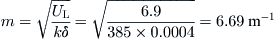
EXAMPLE 3.4
For a collector having the following characteristics and ignoring the bond resistance, calculate the fin efficiency and the collector efficiency factor:
Overall loss coefficient = 6.9 W/m2 °C.
Tube outside diameter = 15 mm.
Tube inside diameter = 13.5 mm.
Heat transfer coefficient inside the tubes = 320 W/m2 °C.
Solution
From Table A5.3, in Appendix 5, for copper, k = 385 W/m °C.
From Eq. (3.34),
From Eq. (3.42),

Finally, from Eq. (3.48) and ignoring bond conductance,

3.3.4 Heat removal factor, flow factor, and thermal efficiency
Consider an infinitesimal length δy of the tube as shown in Figure 3.31. The useful energy delivered to the fluid is ![]()
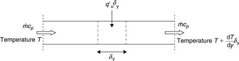
FIGURE 3.31 Energy flow through an element of riser tube.
Under steady-state conditions, an energy balance for n tubes gives:
![]() (3.50)
(3.50)
Dividing through by δy, finding the limit as δy approaches 0, and substituting Eq. (3.47) results in the following differential equation:
![]() (3.51)
(3.51)
Separating variables gives:
Assuming variables F′, UL, and cp to be constants and performing the integrations gives:
![]() (3.53)
(3.53)
The quantity nWL in Eq. (3.53) is the collector area Ac. Therefore,
![]() (3.54)
(3.54)
It is usually desirable to express the collector total useful energy gain in terms of the fluid inlet temperature. To do this the collector heat removal factor needs to be used. Heat removal factor represents the ratio of the actual useful energy gain that would result if the collector-absorbing surface had been at the local fluid temperature. Expressed symbolically:
![]() (3.55)
(3.55)
or
![]() (3.56)
(3.56)
Rearranging yields:
![]() (3.57)
(3.57)
Introducing Eq. (3.54) into Eq. (3.57) gives:
![]() (3.58)
(3.58)
Another parameter usually used in the analysis of collectors is the flow factor. This is defined as the ratio of FR to F′, given by:
![]() (3.59)
(3.59)
As shown in Eq. (3.59), the collector flow factor is a function of only a single variable, the dimensionless collector capacitance rate, ![]() , shown in Figure 3.32.
, shown in Figure 3.32.
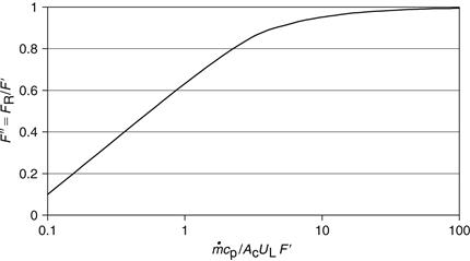
FIGURE 3.32 Collector flow factor as a function of the dimensionless capacitance rate.
If we replace the nominator of Eq. (3.56) with Qu and S with Gt(τα) from Eq. (3.6), then the following equation is obtained:
![]() (3.60)
(3.60)
This is the same as Eq. (3.31), with the difference that the inlet fluid temperature (Ti) replaces the average plate temperature (Tp) with the use of the FR.
In Eq. (3.60), the temperature of the inlet fluid, Ti, depends on the characteristics of the complete solar heating system and the hot water demand or heat demand of the building. However, FR is affected only by the solar collector characteristics, the fluid type, and the fluid flow rate through the collector.
From Eq. (3.60), the critical radiation level can also be defined. This is the radiation level where the absorbed solar radiation and loss term are equal. This is obtained by setting the term in the right-hand side of Eq. (3.60) equal to 0 (or Qu = 0). Therefore, the critical radiation level, Gtc, is given by:
![]() (3.61)
(3.61)
As in the collector performance tests, described in Chapter 4, the parameters obtained are the FRUL and FR(τα), it is preferable to keep FR in Eq. (3.61). The collector can provide useful output only when the available radiation is higher than the critical one. The collector output can be written in terms of the critical radiation level as Qu = AcFR(τα)(Gt − Gtc)+, which implies that the collector produces useful output only when the absorbed solar radiation is bigger than the thermal losses and Gt is greater than Gtc.
Finally, the collector efficiency can be obtained by dividing Qu, Eq. (3.60), by (GtAc). Therefore,
![]() (3.62)
(3.62)
For incident angles below about 35°, the product τ × α is essentially constant and Eqs (3.60) and (3.62) are linear with respect to the parameter (Ti − Ta)/Gt, as long as UL remains constant.
To evaluate the collector tube inside heat transfer coefficient, hfi, the mean absorber temperature, Tp, is required. This can be found by solving Eqs (3.60) and (3.31) simultaneously, which gives:
EXAMPLE 3.5
For the collector outlined in Example 3.4, calculate the useful energy and the efficiency if collector area is 4 m2, flow rate is 0.06 kg/s, (τα) = 0.8, the global solar radiation for 1 h is 2.88 MJ/m2, and the collector operates at a temperature difference of 5 °C.
Solution
The dimensionless collector capacitance rate is:
From Eq. (3.59),
Therefore, the heat removal factor is (F′ = 0.912 from Example 3.4):

From Eq. (3.60) modified to use It instead of Gt,

and the collector efficiency is:

3.3.5 Serpentine collector
The analysis presented in Section 3.3.3 concerns the fin and tube assembly in a riser header configuration. The same analysis applies also for a serpentine collector configuration, shown in the right side of Figure 3.1(a), if the pipes are fixed to separate fins as before. If, however, the absorber plate is a continuous plate then a reduced performance is obtained and the analysis is more complicated. The original analysis of this arrangement for a single bend (N) was made by Abdel-Khalik (1976) and subsequently Zhang and Lavan (1985) gave an analysis for up to four bends. In this analysis the heat removal factor, FR, is given in terms of various dimensionless parameters as follows:
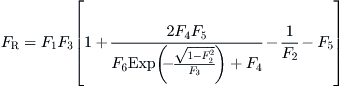 (3.64a)
![]() (3.64b)
(3.64b)
![]() (3.64c)
(3.64c)
![]() (3.64d)
(3.64d)
![]() (3.64e)
(3.64e)
![]() (3.64f)
(3.64f)
![]() (3.64g)
(3.64g)
![]() (3.64h)
(3.64h)
![]() (3.64i)
(3.64i)
![]() (3.64j)
(3.64j)
![]() (3.64k)
(3.64k)
It should be noted that m is given by Eq. (3.34) and Cb is given by Eq. (3.46). Recognizing that Ac is equal to NWL, Eq. (3.64b) can be written as:
![]() (3.65a)
(3.65a)
Similarly, by applying Eq. (3.34) for m and applying Eq. (3.64i) to Eq. (3.64h):
![]() (3.65b)
(3.65b)
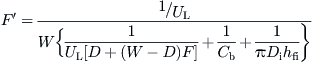
Finally, a more simplified form of Eq. (3.64a) can be obtained by applying Eq. (3.64e) and performing some simple modifications:
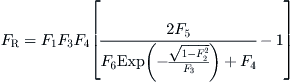 (3.66)
3.3.6 Heat losses from unglazed collectors
When no glazing is used in a flat-plate collector there is no transmittance loss but the radiation and convection losses become very important. In this case the basic performance equation, by ignoring the ground-reflected radiation, is given by:
![]() (3.67)
(3.67)
By adding and subtracting ![]() to the last term and performing some simple manipulations we get:
to the last term and performing some simple manipulations we get:
![]() (3.68a)
(3.68a)
or
![]() (3.68b)
(3.68b)
where
![]() (3.68c)
(3.68c)
![]() (3.68d)
(3.68d)
![]() (3.68e)
(3.68e)
The term GL given by Eq. (3.68d) is the longwave radiation exchange between the absorber and the sky. It should be noted that if the back and end losses from the collector are important, these should be added to the term UL, although their magnitude is much lower than the convection and radiation losses. The efficiency can be obtained by diving Eq. (3.68b) by AcGt, which gives:
![]() (3.69a)
(3.69a)
or
![]() (3.69b)
(3.69b)
where
![]() (3.69c)
(3.69c)
The parameter Gn is called the net incident radiation. Typical values of ε/α are about 0.95.
By relating the sky emissivity in terms of ambient temperature, for clear sky conditions, Eq. (3.68d) becomes (Morrison, 2001):

Leave a Reply