When estimating the building thermal load, adequate results can be obtained by calculating heat losses and gains based on a steady-state heat transfer analysis. For more accurate results and for energy analysis, however, transient analysis must be employed, since the heat gain into a conditioned space varies greatly with time, primarily because of the strong transient effects created by the hourly variation of a solar radiation. Many methods can be used to estimate the thermal load of buildings. The most well-known are the heat balance, weighting factors, thermal network, and radiant time series. In this book, only the heat balance method is briefly explained. Additionally, the degree-day method, which is a more simplified one used to determine the seasonal energy consumption, is described. Before proceeding, however, the three basic terms that are important in thermal load estimation are explained.
Heat gain
Heat gain is the rate at which energy is transferred to or generated within a space and consists of sensible and latent gain. Heat gains usually occur in the following forms:
1. Solar radiation passing through glazing and other openings;
2. Heat conduction with convection and radiation from the inner surfaces into the space;
3. Sensible heat convection and radiation from internal objects;
4. Ventilation and infiltration; and
5. Latent heat gains generated within the space.
Thermal load
The thermal load is the rate at which energy must be added or removed from a space to maintain the temperature and humidity at the design values.
The cooling load differs from the heat gain mainly because the radiant energy from the inside surfaces, as well as the direct solar radiation passing into a space through openings, is mostly absorbed in the space. This energy becomes part of the cooling load only when the room air receives the energy by convection and occurs when the various surfaces in the room attain higher temperatures than the room air. Hence, there is a time lag that depends on the storage characteristics of the structure and interior objects and is more significant when the heat capacity (product of mass and specific heat) is greater. Therefore, the peak cooling load can be considerably smaller than the maximum heat gain and occurs much later than the maximum heat gain period. The heating load behaves in a similar manner as the cooling load.
Heat extraction rate
The heat extraction rate is the rate at which energy is removed from the space by cooling and dehumidifying equipment. This rate is equal to the cooling load when the space conditions are constant and the equipment is operating. Since the operation of the control systems induces some fluctuation in the room temperature, the heat extraction rate fluctuates and this also causes fluctuations in the cooling load.
6.1.1 The heat balance method
The heat balance method is able to provide dynamic simulations of the building load. It is the foundation for all calculation methods that can be used to estimate the heating and cooling loads. Since all energy flows in each zone must be balanced, a set of energy balance equations for the zone air and the interior and exterior surfaces of each wall, roof, and floor must be solved simultaneously. The energy balance method combines various equations, such as equations for transient conduction heat transfer through walls and roofs, algorithms or data for weather conditions, and internal heat gains.
The method can be illustrated by considering a zone consisting of six surfaces, four walls, a roof, and a floor. The zone receives energy from solar radiation coming through windows, heat conducted through exterior walls and the roof, and internal heat gains due to lighting, equipment, and occupants. The heat balance on each of the six surfaces is generally represented by:
![]() (6.1)
(6.1)
qi,θ = rate of heat conducted into surface i at the inside surface at time θ (W);
ns = number of surfaces in the room;
hci = convective heat transfer coefficient at interior of surface i (W/m2 K);
gij = linearized radiation heat transfer factor between interior surface i and interior surface j (W/m2 K);
tα,θ = inside air temperature at time θ (°C);
ti,θ = average temperature of interior surface i at time θ (°C);
tj,θ = average temperature of interior surface j at time θ (°C);
qsi,θ = rate of solar heat coming through the windows and absorbed by surface i at time θ (W);
qli,θ = rate of heat from the lighting absorbed by surface i at time θ (W); and
qei,θ = rate of heat from equipment and occupants absorbed by surface i at time θ (W).
The equations governing a conduction within the six surfaces cannot be solved independent of Eq. (6.1), since the energy exchanges occurring within the room affect the inside surface conditions, which in turn affect the internal conduction. Consequently, the aforementioned six formulations of Eq. (6.1) must be solved simultaneously with the equations governing conduction within the six surfaces to calculate the space thermal load. Among the possible ways to model this process are numerical finite element and time series methods. Most commonly, due to the greater computational speed and little loss of generality, conduction within the structural elements is formulated using conduction transfer functions (CTFs) in the general form:
![]() (6.2)
(6.2)
M = the number of non-zero CTF values;
o = outside surface subscript;
Fm = flux history coefficients.
Conduction transfer function coefficients generally are referred to as response factors and depend on the physical properties of the wall or roof materials and the scheme used for calculating them. These coefficients relate an output function at a given time to the value of one or more driving functions at a given time and at a set period immediately preceding (ASHRAE, 2005). The Y (cross-CTF) values refer to the current and previous flows of energy through the wall due to the outside conditions, the Z (interior CTF) values refer to the internal space conditions, and the Fm (flux history) coefficients refer to the current and previous heat flux to zone.
Equation (6.2), which utilizes the transfer function concept, is a simplification of the strict heat balance calculation procedure, which could be used in this case for calculating conduction heat transfer.
It must be noted that the interior surface temperature ti,θ is present in both Eqs (6.1) and (6.2), and therefore a simultaneous solution is required. In addition, the equation representing the energy balance on the zone air must also be solved simultaneously. This can be calculated from the cooling load equation:
![]() (6.3)
(6.3)
tα,θ = inside air temperature at time θ (°C);
to,θ = outdoor air temperature at time θ (°C);
tv,θ = ventilation air temperature at time θ (°C);
cp = specific heat of air (J/kg K);
Qi,θ = volume flow rate of outdoor air infiltrating into the room at time θ (m3/s);
Qv,θ = volume rate of flow of ventilation air at time θ (m3/s);
Qs,θ = rate of solar heat coming through the windows and convected into the room air at time θ (W);
ql,θ = rate of heat from the lights convected into the room air at time θ (W); and
qe,θ = rate of heat from equipment and occupants convected into the room air at time θ (W).
6.1.2 The transfer function method
The ASHRAE Task Group on Energy Requirements developed the general procedure referred to as the transfer function method (TFM). This approach is a method that simplifies the calculations, can provide the loads originating from various parts of the building, and can be used to determine the heating and cooling loads.
The method is based on a series of conduction transfer functions (CTFs) and a series of room transfer functions (RTFs). The CTFs are used for calculating wall or roof heat conduction; the RTFs are used for load elements that have radiant components, such as lights and appliances. These functions are response time series, which relate a current variable to the past values of itself and other variables in periods of 1 h.
Wall and roof transfer functions
Conduction transfer functions are used by the TFM to describe the heat flux at the inside of a wall, roof, partition, ceiling, and floor. Combined convection and radiation coefficients on the inside (8.3 W/m2 K) and outside surfaces (17.0 W/m2 K) are utilized by the method. The approach uses sol–air temperatures to represent outdoor conditions and assumes constant indoor air temperature. Thus, the heat gain though a wall or roof is given by:
![]() (6.4)
(6.4)
qe,θ = heat gain through wall or roof, at calculation hour θ (W);.
A = indoor surface area of wall or roof (m2);
n = summation index (each summation has as many terms as there are non-negligible values of coefficients);
te,θ−nδ = sol–air temperature at time θ−nδ (°C);
trc = constant indoor room temperature (°C); and
bn, cn, dn = conduction transfer function coefficients.
Conduction transfer function coefficients depend only on the physical properties of the wall or roof. These coefficients are given in tables (ASHRAE, 1997). The b and c coefficients must be adjusted for the actual heat transfer coefficient (Uactual) by multiplying them with the ratio Uactual/Ureference.
In Eq. (6.4), a value of the summation index n equal to 0 represents the current time interval, n equal to 1 is the previous hour, and so on.
The sol–air temperature is defined as:
![]() (6.5)
(6.5)
te = sol–air temperature (°C);
t0 = current hour dry-bulb temperature (°C);
α = absorptance of surface for solar radiation;
Gt = total incident solar load (W/m2);
δR = difference between longwave radiation incident on the surface from the sky and surroundings and the radiation emitted by a blackbody at outdoor air temperature (W/m2);
h0 = heat transfer coefficient for convection over the building (W/m2 K); and
εδR/h0 = longwave radiation factor = −3.9 °C for horizontal surfaces, 0 °C for vertical surfaces.
The term α/h0 in Eq. (6.5) varies from about 0.026 m2 K/W for a light-colored surface to a maximum of about 0.053 m2 K/W. The heat transfer coefficient for convection over the building can be estimated from:
![]() (6.6)
(6.6)
where h0 is in W/m2 K and V is the wind speed in m/s.
Partitions, ceilings, and floors
Whenever a conditioned space is adjacent to other spaces at different temperatures, the transfer of heat through the partition can be calculated from Eq. (6.4) by replacing the sol–air temperature with the temperature of the adjacent space.
When the air temperature of the adjacent space (tb) is constant or the variations of this temperature are small compared to the difference of the adjacent space and indoor temperature difference, the rate of heat gains (qp) through partitions, ceilings, and floors can be calculated from the formula:
![]() (6.7)
(6.7)
A = area of element under analysis (m2);
U = overall heat transfer coefficient (W/m2 K); and
(tb − ti) = adjacent space–indoor temperature difference (°C).
Glazing
The total rate of heat admission through glass is the sum of the transmitted solar radiation, the portion of the absorbed radiation that flows inward, and the heat conducted through the glass whenever there is an outdoor–indoor temperature difference. The rate of heat gain (qs) resulting from the transmitted solar radiation and the portion of the absorbed radiation that flows inward is:
![]() (6.8)
(6.8)
A = area of element under analysis (m2);
SHGC = solar heat-gain coefficient, varying according to orientation, latitude, hour, and month.
The rate of conduction heat gain (q) is:
![]() (6.9)
(6.9)
A = area of element under analysis (m2);
U = glass heat transfer coefficient (W/m2 K); and
(to − ti) = outdoor–indoor temperature difference (°C).
People
The heat gain from people is in the form of sensible and latent heat. The latent heat gains are considered as instantaneous loads. The total sensible heat gain from people is not converted directly to cooling load. The radiant portion is first absorbed by the surroundings and convected to the space at a later time, depending on the characteristics of the room. The ASHRAE Handbook of Fundamentals (2005) gives tables for various circumstances and formulates the gains for the instantaneous sensible cooling load as:
![]() (6.10)
(6.10)
qs = rate of sensible cooling load due to people (W);
SHGp = sensible heat gain per person (W/person).
The rate of latent cooling load is:
![]() (6.11)
(6.11)
ql = latent cooling load due to people (W);
LHGp = latent heat gain per person (W/person).
Lighting
Generally, lighting is often a major internal load component. Some of the energy emitted by the lights is in the form of radiation that is absorbed in the space and transferred later to the air by convection. The manner in which the lights are installed, the type of air distribution system, and the mass of the structure affect the rate of heat gain at any given moment. Generally, this gain can be calculated from:
![]() (6.12)
(6.12)
qel = rate of heat gain from lights (W);
Wl = total installed light wattage (W);
Ful = lighting use factor, ratio of wattage in use to total installed wattage; and
Fsa = special allowance factor (ballast factor in the case of fluorescent and metal halide fixtures).
Appliances
Considerable data are available for this category of cooling load, but careful evaluation of the operating schedule and the load factor for each piece of equipment is essential. Generally, the sensible heat gains from the appliances (qa) can be calculated from:
![]() (6.13)
(6.13)
or
![]() (6.14)
(6.14)
Wa = rate of energy input from appliances (W);
FU, FR, FL = usage factors, radiation factors, and load factors.
Ventilation and infiltration air
Both sensible (qs,v) and latent (ql,v) rates of heat gain result from the incoming air, which may be estimated from:
![]() (6.15)
(6.15)
![]() (6.16)
(6.16)
ma = air mass flow rate (kg/s);
cp = specific heat of air (J/kg K);
(to − ti) = temperature difference between incoming and room air (°C);
(ωo − ωi) = humidity ratio difference between incoming and room air (kg/kg); and
ifg = enthalpy of evaporation (J/kg K).
6.1.3 Heat extraction rate and room temperature
The cooling equipment, in an ideal case, must remove heat energy from the space’s air at a rate equal to the cooling load. In this way, the space air temperature will remain constant. However, this is seldom true. Therefore, a transfer function has been devised to describe the process. The room air transfer function is:
![]() (6.17)
(6.17)
pi, gi = transfer function coefficients (ASHRAE, 1992);
qx = heat extraction rate (W);
qc = cooling load at various times (W);
ti = room temperature used for cooling load calculations (°C); and
tr = actual room temperature at various times (°C).
All g coefficients refer to a unit floor area. The coefficients g0 and gi depend also on the average heat conductance to the surroundings (UA) and the infiltration and ventilation rate to the space. The p coefficients are dimensionless.
The characteristic of the terminal unit usually is of the form:
![]() (6.18)
(6.18)
where W and S are parameters that characterize the equipment at time θ.
The equipment being modeled is actually the cooling coil and the associated control system (thermostat) that matches the coil load to the space load. The cooling coil can extract heat energy from the space air from some minimum to some maximum value.
Equations (6.17) and (6.18) may be combined and solved for qx,θ:
![]() (6.19)
(6.19)
where
![]() (6.20)
(6.20)
When the value of qx,θ computed by Eq. (6.19) is greater than qx,max, it is taken to be equal to qx,max; when it is less than qx,min, it is made equal to qx,min. Finally, Eqs (6.18) and (6.19) can be combined and solved for tr,θ:
![]() (6.21)
(6.21)
It should be noted that, although it is possible to perform thermal load estimation manually with both the heat balance and the transfer function methods, these are better suited for computerized calculation, due to the large number of operations that need to be performed.
6.1.4 Degree-day method
Frequently, in energy calculations, simpler methods are required. One such simple method, which can give comparatively accurate results, is the degree-day method. This method is used to predict the seasonal energy consumption. Each degree that the average outdoor air temperature falls below a balance temperature, Tb, of 18.3 °C (65 °F) represents a degree day. The number of degree days in a day is obtained approximately by the difference of Tb and the average outdoor air temperature, Tav, defined as (Tmax + Tmin)/2. Therefore, if the average outdoor air temperature of a day is 15.3 °C, the number of heating degree-days (DD)h for the day is 3. The number of heating degree-days over a month is obtained by the sum of the daily values (only positive values are considered) from:
![]() (6.22)
(6.22)
Similarly, cooling degree-days are obtained from:
![]() (6.23)
(6.23)
Degree days for both heating (DD)h and cooling (DD)c are published by the meteorological services of many countries. Appendix 7 lists the values of both heating and cooling degree-days for a number of countries. Using the degree-days’ concept, the following equation can be used to determine the monthly or seasonal heating load or demand (Dh):
![]() (6.24)
(6.24)
where UA represents the heat loss characteristic of the building, given by:
![]() (6.25)
(6.25)
Qh = design rate or sensible heat loss (kW);
Ti − To = design indoor–outdoor temperature difference (°C).
Substituting Eq. (6.25) into (6.24) and multiplying by 3600 × 24 = 86,400 to convert days into seconds, the following equation can be obtained for the monthly or seasonal heating load or demand in kJ:
![]() (6.26)
(6.26)
For cooling, the balance temperature is usually 24.6 °C. Similar to the preceding, the monthly or seasonal cooling load or demand in kJ is given by:
EXAMPLE 6.1
A building has a peak heating load equal to 15.6 kW and a peak cooling load of 18.3 kW. Estimate the seasonal heating and cooling requirements if the heating degree-days are 1020 °C days, the cooling degree-days are 870 °C days, the winter indoor temperature is 21 °C, and the summer indoor temperature is 26 °C. The design outdoor temperature for winter is 7 °C and for summer is 36 °C.
Solution
Using Eq. (6.26), the heating requirement is:

Similarly, for the cooling requirement, Eq. (6.27) is used:

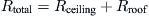
6.1.5 Building heat transfer
The design of space-heating or cooling systems for a building requires the determination of the building thermal resistance. Heat is transferred in building components by all modes: conduction, convection, and radiation. In an electrical analogy, the rate of heat transfer through each building component can be obtained from:
![]() (6.28)
(6.28)
ΔTtotal = total temperature difference between inside and outside air (K);
Rtotal = total thermal resistance across the building element, = ![]() ; and
; and
A = area of the building element perpendicular to the heat flow direction (m2).
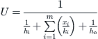
It is obvious from Eq. (6.28) that the overall heat transfer coefficient, U, is equal to:
![]() (6.29)
(6.29)
As in a collector heat transfer, described in Chapter 3, it is easier to apply an electrical analogy to evaluate the building thermal resistances. For conduction heat transfer through a wall element of thickness x (m) and thermal conductivity k (W/m K), the thermal resistance, based on a unit area, is:
![]() (6.30)
(6.30)
The thermal resistance per unit area for convection and radiation heat transfer, with a combined convection and radiation heat transfer coefficient h (W/m2 K), is:
![]() (6.31)
(6.31)
Figure 6.1 illustrates a single-element wall. The thermal resistance due to conduction through the wall is x/k, Eq. (6.30), and the thermal resistance at the inside and outside boundaries of the wall are 1/hi and 1/ho, Eq. (6.31), respectively. Therefore, from the preceding discussion, the total thermal resistance based on the inside and outside temperature difference is the sum of the three resistances as:
![]() (6.32)
(6.32)
or
![]() (6.33)
(6.33)
The values of hi, ho, and k can be obtained from handbooks (e.g. ASHRAE, 2005). Values for typical materials are shown in Table A5.4 and for stagnant air and surface resistance in Table A5.5 in Appendix 5. For multilayer or composite walls like the one shown in Figure 6.2, the following general equation can be used:
 (6.34)
m = number of materials of the composite construction.
For the particular case shown in Figure 6.2, where three layers of materials are used, the following equation applies:
![]() (6.35)
(6.35)
It should be noted that small thickness layers, like paints and glues, are often ignored from this calculation.
EXAMPLE 6.2
Find the overall heat transfer coefficient of the construction shown in Figure 6.2 if components 1 and 3 are brick 10 cm in thickness and the center one is stagnant air 5 cm in thickness. Additionally, the wall is plastered with 25 mm plaster on each side.
Solution
Using the data shown in Tables A5.4 and A5.5 in Appendix 5, we get the following list of resistance values:
1. Outside surface resistance = 0.044.
2. Plaster 25 mm = 0.025/1.39 = 0.018.
3. Brick 10 cm = 0.10/0.25 = 0.4.
5. Brick 10 cm = 0.10/0.25 = 0.4.
6. Plaster 25 mm = 0.025/1.39 = 0.018.
7. Inside surface resistance = 0.12.
Total resistance = 1.18 m2 K/W or U = 1/1.18 = 0.847 W/m2 K.
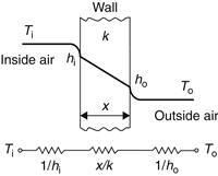
FIGURE 6.1 Heat transfer through a building element and equivalent electric circuit.
FIGURE 6.2 Multilayer wall heat transfer.
In some countries minimum U values for the various building components are specified by law to prohibit building poorly insulated buildings, which require a lot of energy for their heating and cooling needs.
Another situation usually encountered in buildings is the pitched roof shown in Figure 6.3.
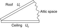
FIGURE 6.3 Pitched roof arrangement.
Using the electrical analogy, the combined thermal resistance is obtained from:
![]() (6.36)
(6.36)
which gives:
![]() (6.37)
(6.37)
UR = combined overall heat transfer coefficient for the pitched roof (W/m2 K);
Uc = overall heat transfer coefficient for the ceiling per unit area of the ceiling (W/m2 K);
Ur = overall heat transfer coefficient for the roof per unit area of the roof (W/m2 K);
Leave a Reply