
The f-chart method is used for estimating the annual thermal performance of active building heating systems using a working fluid, which is either liquid or air, and where the minimum temperature of energy delivery is near 20 °C. The system configurations that can be evaluated by the f-chart method are common in residential applications. With the f-chart method, the fraction of the total heating load that can be supplied by the solar energy system can be estimated. Let the purchased energy for a fuel-only system or the energy required to cover the load be L, the purchased auxiliary energy for a solar system be LAUX, and the solar energy delivered be QS. For a solar energy system, L = LAUX + QS. For a month, i, the fractional reduction of purchased energy when a solar energy system is used, called the solar fraction, f, is given by the ratio:
The f-chart method was developed by Klein et al. (1976, 1977) and Beckman et al. (1977). In the method, the primary design variable is the collector area, while the secondary variables are storage capacity, collector type, load and collector heat-exchanger size, and fluid flow rate. The method is a correlation of the results of many hundreds of thermal performance simulations of solar heating systems performed with TRNSYS, in which the simulation conditions were varied over specific ranges of parameters of practical system designs shown in Table 11.1 (Klein et al., 1976, 1977). The resulting correlations give f, i.e., the fraction of the monthly load supplied by solar energy, as a function of two dimensionless parameters. The first is related to the ratio of collector losses to heating load, and the second to the ratio of absorbed solar radiation to heating load. The heating load includes both space heating and hot water loads. The f-chart method has been developed for three standard system configurations: liquid and air systems for space and hot water heating and systems for service hot water only.
Table 11.1
Range of Design Variables Used in Developing f-Charts for Liquid and Air Systems
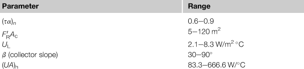
Reprinted from Klein et al. (1976, 1977), with permission from Elsevier.
Based on the fundamental equation presented in Chapter 6, Section 6.3.3, Klein et al. (1976) analyzed numerically the long-term thermal performance of solar heating systems of the basic configuration shown in Figure 6.14. When Eq. (6.60) is integrated over a time period, Δt, such that the internal energy change in the storage tank is small compared to the other terms (usually one month), we get:
![]() (11.2)
(11.2)
The sum of the last three terms of Eq. (11.2) represents the total heating load (including space load and hot water load) supplied by solar energy during the integration period. If this sum is denoted by QS, using the definition of the solar fraction, f, from Eq. (11.1), we get:
![]() (11.3)
(11.3)
where L = total heating load during the integration period (MJ).
Using Eq. (5.56) for Qu and replacing Gt by Ht, the total (beam and diffuse) insolation over a day, Eq. (11.3) can be written as:
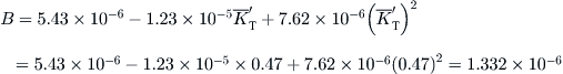
The last term of Eq. (11.4) can be multiplied and divided by the term (Tref − Ta), where Tref is a reference temperature chosen to be 100 °C, so the following equation can be obtained:
![]() (11.5)
(11.5)
The storage tank temperature, Ts, is a complicated function of Ht, L, and Ta; therefore, the integration of Eq. (11.5) cannot be explicitly evaluated. This equation, however, suggests that an empirical correlation can be found, on a monthly basis, between the f factor and the two dimensionless groups mentioned above as follows:
![]() (11.6)
(11.6)
![]() (11.7)
(11.7)
L = monthly heating load or demand (MJ);
N = number of days in a month;
![]() = monthly average ambient temperature (°C);
= monthly average ambient temperature (°C);
![]() = monthly average daily total radiation on the tilted collector surface (MJ/m2); and
= monthly average daily total radiation on the tilted collector surface (MJ/m2); and
![]() = monthly average value of (τα), = monthly average value of absorbed over incident solar radiation =
= monthly average value of (τα), = monthly average value of absorbed over incident solar radiation = ![]() .
.
For the purpose of calculating the values of the dimensionless parameters X and Y, Eqs (11.6) and (11.7) are usually rearranged to read:
![]() (11.8)
(11.8)
![]() (11.9)
(11.9)
The reason for the rearrangement is that the factors FRUL and FR(τα)n are readily available from standard collector tests (see Chapter 4, Section 4.1). The ratio ![]() corrects the collector performance because a heat exchanger is used between the collector and the storage tank, which causes the collector side of the system to operate at higher temperature than a similar system without a heat exchanger and is given by Eq. (5.57) in Chapter 5. For a given collector orientation, the value of the factor
corrects the collector performance because a heat exchanger is used between the collector and the storage tank, which causes the collector side of the system to operate at higher temperature than a similar system without a heat exchanger and is given by Eq. (5.57) in Chapter 5. For a given collector orientation, the value of the factor ![]() varies slightly from month to month. For collectors tilted and facing the equator with a slope equal to latitude plus 15°, Klein (1976) found that the factor is equal to 0.96 for a one-cover collector and 0.94 for a two-cover collector for the whole heating season (winter months). Using the preceding definition of
varies slightly from month to month. For collectors tilted and facing the equator with a slope equal to latitude plus 15°, Klein (1976) found that the factor is equal to 0.96 for a one-cover collector and 0.94 for a two-cover collector for the whole heating season (winter months). Using the preceding definition of ![]() , we get:
, we get:
If the isotropic model is used for ![]() and substituted in Eq. (11.10), then:
and substituted in Eq. (11.10), then:
![]() (11.11)
(11.11)
In Eq. (11.11), the ![]() ratios can be obtained from Figure 3.27 for the beam component at the effective angle of incidence,
ratios can be obtained from Figure 3.27 for the beam component at the effective angle of incidence, ![]() , which can be obtained from Figure A3.8 in Appendix 3, and for the diffuse and ground-reflected components at the effective incidence angles at β from Eqs (3.4a) and (3.4b).
, which can be obtained from Figure A3.8 in Appendix 3, and for the diffuse and ground-reflected components at the effective incidence angles at β from Eqs (3.4a) and (3.4b).
The dimensionless parameters, X and Y, have some physical significance. The parameter X represents the ratio of the reference collector total energy loss to total heating load or demand (L) during the period Δt, whereas the parameter Y represents the ratio of the total absorbed solar energy to the total heating load or demand (L) during the same period.
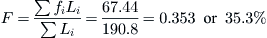
As was indicated, f-chart is used to estimate the monthly solar fraction, fi, and the energy contribution for the month is the product of fi and monthly load (heating and hot water), Li. To find the fraction of the annual load supplied by the solar energy system, F, the sum of the monthly energy contributions is divided by the annual load, given by:
![]() (11.12)
(11.12)
The method can be used to simulate standard solar water and air system configurations and solar energy systems used only for hot water production. These are examined separately in the following sections.
EXAMPLE 11.1
A standard solar-heating system is installed in an area where the average daily total radiation on the tilted collector surface is 12.5 MJ/m2, average ambient temperature is 10.1 °C, and it uses a 35 m2 aperture area collector, which has FR(τα)n = 0.78 and FRUL = 5.56 W/m2 °C, both determined from the standard collector tests. If the space heating and hot water load is 35.2 GJ, the flow rate in the collector is the same as the flow rate used in testing the collector, ![]() , and
, and ![]() for all months, estimate the parameters X and Y.
for all months, estimate the parameters X and Y.
Solution
Using Eqs (11.8) and (11.9) and noting that ΔT is the number of seconds in a month, equal to 31 days × 24 h × 3600 s/h, we get:


It should be noted that F′RUL and F′R(τα)n can be given instead of FRUL, FR(τα)n and F′R/FR, given in this problem.
11.1.1 Performance and design of liquid-based solar heating systems
Knowledge of the system thermal performance is required in order to be able to design and optimize a solar heating system. The f-chart for liquid-based systems is developed for a standard solar liquid-based solar energy system, shown in Figure 11.1. This is the same as the system shown in Figure 6.14, drawn without the controls, for clarity. The typical liquid-based system shown in Figure 11.1 uses an antifreeze solution in the collector loop and water as the storage medium. A water-to-water load-heat exchanger is used to transfer heat from the storage tank to the domestic hot water (DHW) system. Although in Figure 6.14 a one-tank DHW system is shown, a two-tank system could be employed, in which the first tank is used for preheating.
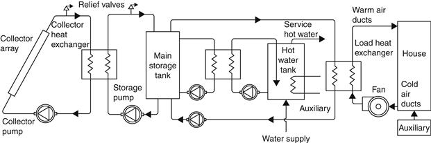
FIGURE 11.1 Schematic diagram of a standard liquid-based solar heating system.
The fraction f of the monthly total load supplied by a standard liquid-based solar energy system is given as a function of the two dimensionless parameters, X and Y, and can be obtained from the f-chart in Figure 11.2 or the following equation (Klein et al., 1976):
![]() (11.13)
(11.13)
Application of Eq. (11.13) or Figure 11.2 allows the simple estimation of the solar fraction on a monthly basis as a function of the system design and local weather conditions. The annual value can be obtained by summing up the monthly values using Eq. (11.12). As will be shown in the next chapter, to determine the economic optimum collector area, the annual load fraction corresponding to different collector areas is required. Therefore, the present method can easily be used for these estimations.
EXAMPLE 11.2
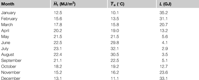
If the solar heating system given in Example 11.1 is liquid-based, estimate the annual solar fraction if the collector is located in an area having the monthly average weather conditions and monthly heating and hot water loads shown in Table 11.2.
Table 11.2
Average Monthly Weather Conditions and Heating and Hot Water Loads for Example 11.2
Solution
The values of the dimensionless parameters X and Y found from Example 11.1 are equal to 1.30 and 0.28, respectively. From the weather and load conditions shown in Table 11.2, these correspond to the month of January. From Figure 11.2 or Eq. (11.13), f = 0.188. The total load in January is 35.2 GJ. Therefore, the solar contribution in January is fL = 0.188 × 35.2 = 6.62 GJ. The same calculations are repeated from month to month, as shown in Table 11.3.
Table 11.3
Monthly Calculations for Example 11.2
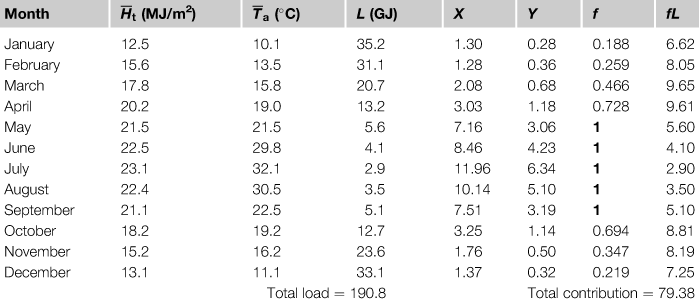
It should be noted that the values of f marked in bold are outside the range of the f-chart correlation and a fraction of 100% is used, as during these months, the solar energy system covers the load fully. From Eq. (11.12), the annual fraction of load covered by the solar energy system is:
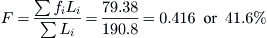
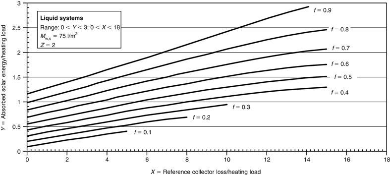
FIGURE 11.2 The f-chart for liquid-based solar heating systems.
It should be noted that the f-chart was developed using fixed nominal values of storage capacity per unit of collector area, collector liquid flow rate per unit of collector area, and load heat-exchanger size relative to a space-heating load. Therefore, it is important to apply various corrections for the particular system configuration used.
Storage capacity correction
It can be proven that the annual performance of liquid-based solar energy systems is insensitive to the storage capacity, as long as this is more than 50 l of water per square meter of collector area. For the f-chart of Figure 11.2, a standard storage capacity of 75 l of stored water per square meter of collector area was considered. Other storage capacities can be used by modifying the factor X by a storage size correction factor Xc/X, given by (Beckman et al., 1977):
![]() (11.14)
(11.14)
Mw,a = actual storage capacity per square meter of collector area (l/m2).
Mw,s = standard storage capacity per square meter of collector area (= 75 l/m2).
Equation (11.14) is applied in the range of 0.5 ≤ (Mw,a/Mw,s) ≤ 4.0 or 37.5 ≤ Mw,a ≤ 300 l/m2. The storage correction factor can also be determined from Figure 11.3 directly, obtained by plotting Eq. (11.14) for this range.
EXAMPLE 11.3
Estimate the solar fraction for the month of March of Example 11.2 if the storage tank capacity is 130 l/m2.
Solution
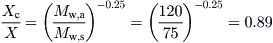
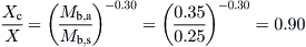
First the storage correction factor needs to be estimated. By using Eq. (11.14),
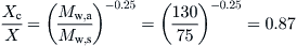
For March, the corrected value of X is then Xc = 0.87 × 2.08 = 1.81. The value of Y remains as estimated before, i.e., Y = 0.68. From the f-chart, f = 0.481 compared to 0.466 before the correction, an increase of about 2%.
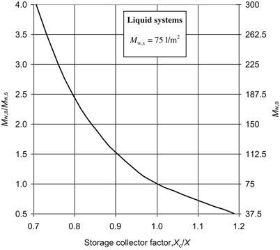
FIGURE 11.3 Storage correction factor for liquid-based systems.
Collector flow rate correction
The f-chart of Figure 11.2 has been generated using a collector antifreeze solution flow rate equal to 0.015 l/s m2. A lower flow rate can reduce the energy collection rate significantly, especially if the low flow rate leads to fluid boiling and relief of pressure through the relief valve. Although the product of the mass flow rate and the specific heat of the fluid flowing through the collector strongly affects the performance of the solar energy system, the value used is seldom lower than the value used for the f-chart development. Additionally, since an increase in the collector flow rate beyond the nominal value has a small effect on the system performance, Figure 11.2 is applicable for all practical collector flow rates.
Load heat exchanger size correction
The size of the load heat exchanger strongly affects the performance of the solar energy system. This is because the rate of heat transfer across the load heat exchanger directly influences the temperature of the storage tank, which consequently affects the collector inlet temperature. As the heat exchanger used to heat the building air is reduced in size, the storage tank temperature must increase to supply the same amount of heat energy, resulting in higher collector inlet temperatures and therefore reduced collector performance. To account for the load heat exchanger size, a new dimensionless parameter is specified, Z, given by (Beckman et al., 1977):
![]() (11.15)
(11.15)
εL = effectiveness of the load heat exchanger.
![]() = minimum mass flow rate–specific heat product of heat exchanger (W/K).
= minimum mass flow rate–specific heat product of heat exchanger (W/K).
(UA)L = building loss coefficient and area product used in degree-day space-heating load model (W/K).
In Eq. (11.15), the minimum capacitance rate is that of the air side of the heat exchanger. System performance is asymptotically dependent on the value of Z; and for Z > 10, the performance is essentially the same as for an infinitely large value of Z. Actually, the reduction in performance due to a small-size load heat exchanger is significant for values of Z lower than 1. Practical values of Z are between 1 and 3, whereas a value of Z = 2 was used for the development of the f-chart of Figure 11.2. The performance of systems having other values of Z can be estimated by multiplying the dimensionless parameter Y by the following correction factor:
![]() (11.16)
(11.16)
Equation (11.16) is applied in the range of 0.5 ≤ Z ≤ 50. The load heat-exchanger size correction factor can also be determined from Figure 11.4 directly, obtained by plotting Eq. (11.16) for this range.
EXAMPLE 11.4
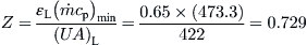
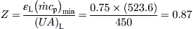
If the liquid flow rate in Example 11.2 is 0.525 l/s, the air flow rate is 470 l/s, the load heat-exchanger effectiveness is 0.65, and the building overall loss coefficient–area product, (UA)L, is 422 W/K, find the effect on the solar fraction for the month of November.
Solution
The minimum value of capacitance needs to be found first. Therefore, if we assume that the operating temperature is 350 K (77 °C) and the properties of air and water at that temperature are as from Tables A5.1 and A5.2 in Appendix 5, respectively,

Therefore, the minimum capacitance is for the air side of the load heat exchanger.
From Eq. (11.15),
The correction factor is given by Eq. (11.16):

From Example 11.2, the value of the dimensionless parameter Y is 0.50. Therefore, Yc = 0.50 × 0.93 = 0.47. The value of the dimensionless parameter X for this month is 1.76, which from Eq. (11.13) gives a solar fraction f = 0.323, a drop of about 2% from the previous value.
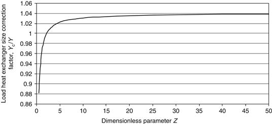
FIGURE 11.4 Load heat exchanger size correction factor.
Although in the examples in this section only one parameter was different from the standard one, if both the storage size and the size of the heat exchanger are different than the standard ones, both Xc and Yc need to be calculated for the determination of the solar fraction. Additionally, most of the required parameters in this section are given as input data. In the following example, most of the required parameters are estimated from the information given in earlier chapters.
EXAMPLE 11.5
A liquid-based solar space and domestic water-heating system is located in Nicosia, Cyprus (35°N latitude). Estimate the monthly and annual solar fraction of the system, which has a total collector area of 20 m2 and the following information is given:
1. The collectors face south, installed with 45° inclination. The performance parameters of the collectors are FR(τα)n = 0.82 and FRUL = 5.65 W/m2 °C, both determined from the standard collector tests.
2. The flow rate of both the water and antifreeze solution through the collector heat exchanger is 0.02 l/s m2 and the factor ![]()
3. The storage tank capacity is equal to 120 l/m2.
4. The ![]() for October through March and 0.93 for April through September.
for October through March and 0.93 for April through September.
5. The building UA value is equal to 450 W/K. The water-to-air load heat exchanger has an effectiveness of 0.75 and air flow rate is 520 l/s.
6. The ground reflectivity is 0.2.
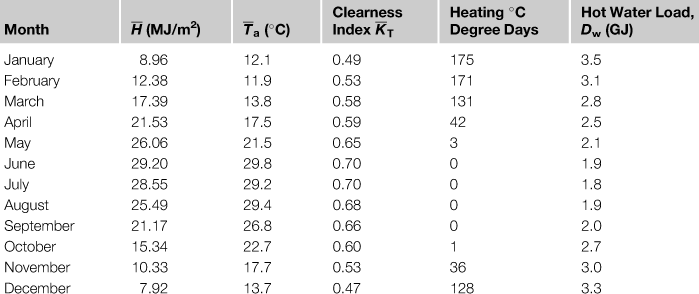
7. The climatic data and the heating degree days for Nicosia, Cyprus, are taken from Appendix 7 and reproduced in Table 11.4 with the hot-water load.
Table 11.4
Climate Data and Heating Degree Days for Example 11.5
Solution
The loads need to be estimated first. For the month of January, from Eq. (6.24):

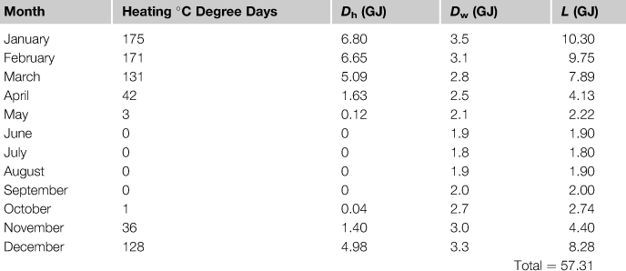
The monthly heating load (including hot-water load) = 6.80 + 3.5 = 10.30 GJ. The results for all the months are shown in Table 11.5.
Table 11.5
Heating Load for All the Months in Example 11.5
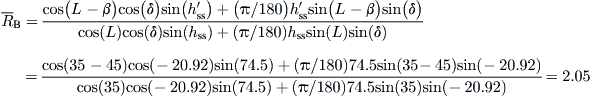
Next, we need to estimate the monthly average daily total radiation on the tilted collector surface from the daily total horizontal solar radiation, ![]() For this estimation, the average day of each month is used, shown in Table 2.1, together with the declination for each day. For each of those days, the sunset hour angle, hss, is required, given by Eq. (2.15), and the sunset hour angle on the tilted surface,
For this estimation, the average day of each month is used, shown in Table 2.1, together with the declination for each day. For each of those days, the sunset hour angle, hss, is required, given by Eq. (2.15), and the sunset hour angle on the tilted surface, ![]() , given by Eq. (2.109). The calculations for the month of January are as follows.
, given by Eq. (2.109). The calculations for the month of January are as follows.
From Eq. (2.15),

From Eq. (2.109),

From Eq. (2.105b),
From Eq. (2.108),
From Eq. (2.107),
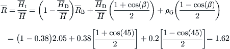
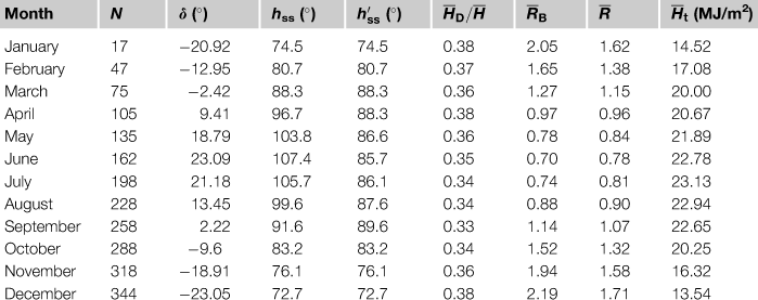
And finally, ![]() The calculations for all months are shown in Table 11.6.
The calculations for all months are shown in Table 11.6.
Table 11.6
Monthly Average Calculations for Example 11.5
We can now move along in the f-chart estimation. The dimensionless parameters X and Y are estimated from Eqs (11.8) and (11.9):


The storage tank correction is obtained from Eq. (11.14):
Then, the minimum capacitance value needs to be found (at an assumed temperature of 77 °C):

Therefore, the minimum capacitance is for the air side of the load heat exchanger.From Eq. (11.15),
The correction factor is given by Eq. (11.16):

Therefore,

and

When these values are used in Eq. (11.13), they give f = 0.419. The complete calculations for all months of the year are shown in Table 11.7.
Table 11.7
Complete Monthly Calculations for the f-Chart for Example 11.5
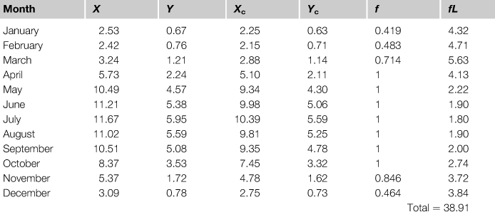
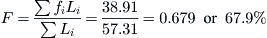
From Eq. (11.12), the annual fraction of load covered by the solar energy system is:
11.1.2 Performance and design of air-based solar heating systems
Klein et al. (1977) developed for air-based systems a design procedure similar to that for liquid-based systems. The f-chart for air-based systems is developed for the standard solar air-based solar energy system, shown in Figure 11.5. This is the same as the system shown in Figure 6.12, drawn without the controls, for clarity. As can be seen, the standard configuration of air-based solar heating system uses a pebble-bed storage unit. The energy required for the DHW is provided through the air-to-water heat exchanger, as shown. During summertime, when heating is not required, it is preferable not to store heat in the pebble bed, so a bypass is usually used, as shown in Figure 11.5 (not shown in Figure 6.12), which allows the use of the collectors for water heating only.
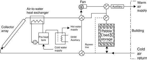
FIGURE 11.5 Schematic diagram of the standard air-based solar heating system.
The fraction f of the monthly total load supplied by a standard solar air-based solar energy system, shown in Figure 11.5, is also given as a function of the two parameters, X and Y, and can be obtained from the f-chart given in Figure 11.6 or from the following equation (Klein et al., 1977):
![]() (11.17)
(11.17)
EXAMPLE 11.6
A solar air-heating system of the standard configuration is installed in the same area as the one in Example 11.2 and the building has the same load. The air collectors have the same area as in Example 11.2 and are double glazed, with FRUL = 2.92 W/m2 °C, FR(τα)n = 0.52, and ![]() Estimate the annual solar fraction.
Estimate the annual solar fraction.
Solution
A general condition of air systems is that no correction factor is required for the collector heat exchanger and ducts are well insulated; therefore, heat losses are assumed to be small, so ![]() . For the month of January and from Eqs (11.8) and (11.9).
. For the month of January and from Eqs (11.8) and (11.9).


From Eq. (11.17) or Figure 11.6, f = 0.147. The solar contribution is fL = 0.147 × 35.2 = 5.17 GJ. The same calculations are repeated for the other months and tabulated in Table 11.8.
Table 11.8
Solar Contribution and f-Values for all Months for Example 11.6
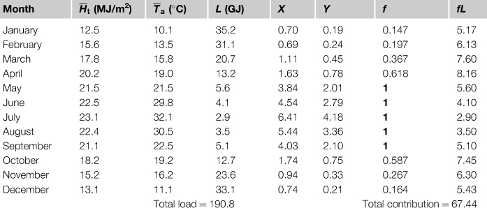
It should be noted here that, again, the values of f marked in bold are outside the range of the f-chart correlation and a fraction of 100% is used because during these months, the solar energy system covers the load fully. From Eq. (11.12), the annual fraction of load covered by the solar energy system is:
Therefore, compared to the results from Example 11.2, it can be concluded that, due to the lower collector optical characteristics, F is lower.
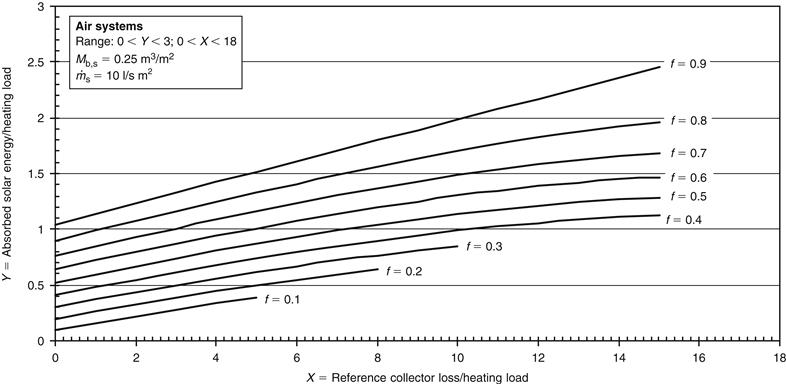
FIGURE 11.6 The f-chart for air-based solar heating systems.
Air systems require two correction factors: one for the pebble-bed storage size and one for the air flow rate, which affects stratification in the pebble bed. There are no load heat exchangers in air systems, and care must be taken to use the collector performance parameters FRUL and FR(τα)n, determined at the same air flow rate as used in the installation; otherwise, the correction outlined in Chapter 4, Section 4.1.1, needs to be used.
Pebble-bed storage size correction
For the development of the f-chart of Figure 11.6, a standard storage capacity of 0.25 cubic meters of pebbles per square meter of collector area was considered, which corresponds to 350 kJ/m2 °C for typical void fractions and rock properties. Although the performance of air-based systems is not as sensitive to the storage capacity as in liquid-based systems, other storage capacities can be used by modifying the factor X by a storage size correction factor, Xc/X, as given by (Klein et al., 1977):
![]() (11.18)
(11.18)
Mb,a = actual pebble storage capacity per square meter of collector area (m3/m2);
Mb,s = standard storage capacity per square meter of collector area = 0.25 m3/m2.
Equation (11.18) is applied in the range of 0.5 ≤ (Mb,a/Mb,s) ≤ 4.0 or 0.125 ≤ Mb,a ≤ 1.0 m3/m2. The storage correction factor can also be determined from Figure 11.7 directly, obtained by plotting Eq. (11.18) for this range.
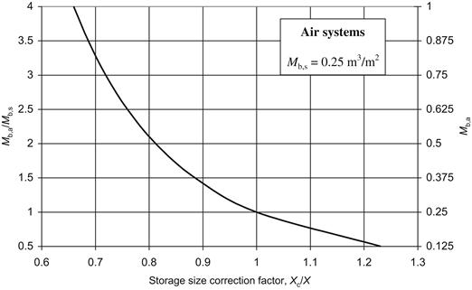
FIGURE 11.7 Storage size correction factor for air-based systems.
Air flow rate correction
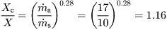
Air-based heating systems must also be corrected for the flow rate. An increased air flow rate tends to increase system performance by improving FR, but it tends to decrease performance by reducing the pebble bed thermal stratification. The standard collector flow rate is 10 l/s of air per square meter of collector area. The performance of systems having other collector flow rates can be estimated by using appropriate values of FR and Y, then modifying the value of X by a collector air flow rate correction factor, Xc/X, to account for the degree of stratification in the pebble bed (Klein et al., 1977):
![]() (11.19)
(11.19)
![]() = actual collector flow rate per square meter of collector area (l/s m2);
= actual collector flow rate per square meter of collector area (l/s m2);
![]() = standard collector flow rate per square meter of collector area = 10 l/s m2.
= standard collector flow rate per square meter of collector area = 10 l/s m2.
Equation (11.19) is applied in the range of ![]() or
or ![]() l/s m2. The air flow rate correction factor can also be determined from Figure 11.8 directly, obtained by plotting Eq. (11.19) for this range.
l/s m2. The air flow rate correction factor can also be determined from Figure 11.8 directly, obtained by plotting Eq. (11.19) for this range.
EXAMPLE 11.7
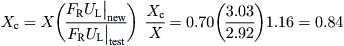
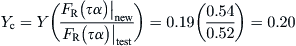
If the air system of Example 11.6 uses a flow rate equal to 17 l/s m2, estimate the solar fraction for the month of January. At the new flow rate, the performance parameters of the collector are FRUL = 3.03 W/m2 °C, FR(τα) = 0.54.
Solution
From Eq. (11.19),
The increased air flow rate also affects the FR and the performance parameters, as shown in the problem definition. Therefore, the value of X to use is the value from Example 11.6 corrected for the new air flow rate through the collector and the pebble bed. Hence,
The dimensionless parameter Y is affected only by the FR. So,
Finally, from the f-chart of Figure 11.6 or Eq. (11.17), f = 0.148 or 14.8%. Compared to the previous result of 14.7%, there is no significant reduction for the increased flow rate, but there will be an increase in fan power.
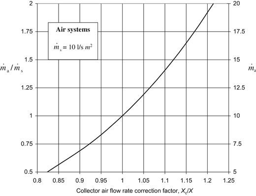
FIGURE 11.8 Correction factor for air flow rate to account for stratification in pebble bed.
If, in a solar energy system, both air flow rate and storage size are different from the standard ones, two corrections must be done on dimensionless parameter X. In this case, the final X value to use is the uncorrected value multiplied by the two correction factors.
EXAMPLE 11.8
If the air system of Example 11.6 uses a pebble storage tank equal to 0.35 m3/m2 and the flow rate is equal to 17 l/s m2, estimate the solar fraction for the month of January. At the new flow rate, the performance parameters of the collector are as shown in Example 11.7.
Solution
The two correction factors need to be estimated first. The correction factors for X and Y for the increased flow rate are as shown in Example 11.7. For the increased pebble bed storage, from Eq. (11.18),
The correction for the air flow rate is given in Example 11.7 and is equal to 1.16. By considering also the correction for the flow rate on FR and the original value of X,

The dimensionless parameter Y is affected only by the FR. So, the value of Example 11.7 is used here (= 0.20). Therefore, from the f-chart of Figure 11.6 or Eq. (11.17), f = 0.153 or 15.3%.
11.1.3 Performance and design of solar service water systems
The f-chart of Figure 11.2 or Eq. (11.13) can also be used to estimate the performance of solar service water-heating systems with a configuration like that shown in Figure 11.9. Although a liquid-based system is shown in Figure 11.9, air or water collectors can be used in the system with the appropriate heat exchanger to transfer heat to the preheat storage tank. Hot water from the preheat storage tank is then fed to a water heater where its temperature can be increased, if required. A tempering valve may also be used to maintain the supply temperature below a maximum temperature, but this mixing can also be done at the point of use by the user.
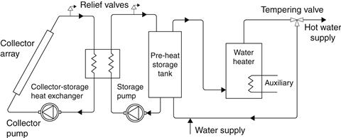
FIGURE 11.9 Schematic diagram of the standard of water-heating system configuration.
The performance of solar water heating systems is affected by the public mains water temperature, Tm, and the minimum acceptable hot water temperature, Tw; both affect the average system operating temperature and thus the collector energy losses. Therefore, the parameter X, which accounts for the collector energy losses, needs to be corrected. The additional correction factor for the parameter X is given by (Beckman et al., 1977):
![]() (11.20)
(11.20)
Tm = mains water temperature (°C);
Tw = minimum acceptable hot water temperature (°C); and
![]() = monthly average ambient temperature (°C).
= monthly average ambient temperature (°C).
The correction factor Xc/X is based on the assumption that the solar preheat tank is well insulated. Tank losses from the auxiliary tank are not included in the f-chart correlations. Therefore, for systems supplying hot water only, the load should also include the losses from the auxiliary tank. Tank losses can be estimated from the heat loss coefficient and tank area (UA) based on the assumption that the entire tank is at the minimum acceptable hot water temperature, Tw.
The solar water heater performance is based on storage capacity of 75 l/m2 of collector aperture area and a typical hot water load profile, with little effect by other distributions on the system performance. For different storage capacities, the correction given by Eq. (11.14) applies.
EXAMPLE 11.9
A solar water heating system is installed in an area where, for the 31-day month under investigation, the average daily total radiation on the tilted collector surface is 19.3 MJ/m2, average ambient temperature is 18.1 °C, and it uses a 5 m2 aperture area collector that has FR(τα)n = 0.79 and FRUL = 6.56 W/m2 °C, both determined from the standard collector tests. The water heating load is 200 l/day, the public mains water temperature, Tm, is 12.5 °C, and the minimum acceptable hot water temperature, Tw, is 60 °C. The storage capacity of the preheat tank is 75 l/m2 and auxiliary tank has a capacity of 150 l, a loss coefficient of 0.59 W/m2 °C, diameter 0.4 m, and height of 1.1 m; it is located indoors, where the environment temperature is 20 °C. The flow rate in the collector is the same as the flow rate used in testing the collector, the ![]() , and the
, and the ![]() Estimate the solar fraction.
Estimate the solar fraction.
Solution
The monthly water-heating load is the energy required to heat the water from Tm to Tw plus the auxiliary tank losses. For the month investigated, the water heating load is:

The auxiliary tank loss rate is given by UA(Tw − Ta). The area of the tank is:

Thus, auxiliary tank loss = 0.59 × 1.63(60 − 20) = 38.5 W. The energy required to cover this loss in a month is:

Therefore,

Using Eqs (11.8) and (11.9), we get:


From Eq. (11.20), the correction for X is:

Therefore, the corrected value of X is:

From Figure 11.2 or Eq. (11.13), for Xc and Y, we get f = 0.808 or 80.8%.
11.1.4 Thermosiphon solar water-heating systems
It is a fact that globally, the majority of solar water heaters installed are of the thermosiphon type. Therefore, it is important to develop a simple method to predict their performance similar to the forced circulation or active systems. This method may be a modification of the original f-chart method presented in the previous sections to account for the natural circulation occurring in thermosiphon systems, which exhibit also a strong stratification of the hot water in the storage tank.
In fact, the original f-chart cannot be used as it is to predict the thermal performance of thermosiphon solar water heaters with good accuracy, for two reasons (Fanney and Klein, 1983; Malkin et al., 1987):
1. The f-chart design tool was developed for pumped systems and the assumption that the fluid flow rate through the collector loop is known and it is fixed. The varying flow rates encountered in thermosiphon solar water-heating systems, driven by the strength of solar radiation, lead to different FR and FRUL values from those encountered in active systems. These parameters are determined experimentally with the procedures outlined in Chapter 4 at fixed flow rate.
2. Additionally, a major assumption made for the development of the f-chart design method is that the hot-water storage tank is fully mixed. Therefore, the thermal performance of thermosiphon solar-water heaters would be greatly underestimated due to the enhanced thermal stratification produced because of the lower mass flow rate from the collector to storage tank. If this is ignored, f-chart would give wrong results leading to system oversizing and would predict reduced cost effectiveness of the thermosiphon solar water-heating system.
The modification to the f-chart design method presented here is suggested by Malkin et al. (1987). In fact they used a correction factor to take into account on the system performance the effect of the enhanced thermal stratification within the hot-water storage tank. This was obtained by using, similarly as in the original f-chart method, a number of TRNSYS simulations for various thermosiphon solar water-heating systems operating in three different locations in the USA (Albuquerque, Madison and Seattle). The characteristics of these three systems are shown in Table 11.9. In addition to these characteristics, in the simulations the overall loss coefficient for the hot-water storage tank was assumed to be constant and equal to 1.46 W/K.
Table 11.9
Range of Design Variables Used in Developing the Modified f-Chart Method for Thermosiphon Units
| Parameter | Range |
| Load draw | 150–500 l |
| Hot-water storage tank size | 100–500 l |
| Collector slope | 30–90° |
| FRUL | 3.6–8.6 W/m2 °C |
| FR(τα) | 0.7–0.8 |
Malkin (1985).
According to Malkin et al. (1987) it is possible to modify the f-chart method to enable prediction of the improved performance of systems exhibiting stratified storage tanks. This can be done by considering the varying flow rate through the thermosiphon system to be approximated by an “equivalent average” fixed flow rate for each month in a corresponding active system of the same size. In this case, the active system operating at this fixed flow rate may yield similar results for monthly fractional energy savings by solar as the thermosiphon system. Therefore, in this way the long-term performance of a thermosiphon system may be easily predicted, using the modified form of the f-chart method but the same chart shown in Figure 11.2 for liquid systems.
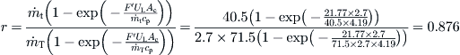
Once the equivalent monthly average fluid flow rate has been calculated from the density differences in the thermosiphon fluid flow loop then the modified values of FR(τα)n and FRUL need to be calculated using the corrective factor (r) given for different test and use flow rates in Chapter 4, Section 4.1.1 by Eq. (4.17) or for the thermosiphon flow in Chapter 5, Section 5.1.1 by Eq. (5.4b) against the normal (or test) flow rate.
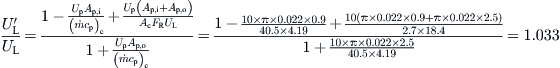
It should be noted that thermally stratified storage tanks return the fluid to the collector at a temperature below that of the average temperature of the storage tank. This results in improved collector efficiency as the temperature entering the collector is lower, closer to ambient and thus the thermal losses from the collector are lower. Thermosiphon systems usually circulate domestic water through the collectors, so they do not include a heat exchanger, therefore by combining Eqs (11.8) and (11.20) the X parameter, called Xmix, is given by:
![]() (11.21)
(11.21)
Similarly the Y parameter without the presence of the heat exchanger term can be given by modifying Eq. (11.9) as:
![]() (11.22)
(11.22)
It should be pointed again that the Xmix and Ymix parameters shown in Eqs (11.21) and (11.22) assume that the hot-water storage tank is fully mixed. Copsey (1984) was the first to develop a modification of the f-chart to account for stratified storage tanks. He has shown that the solar fraction of a stratified tank system (f) can be obtained by analyzing an otherwise identical fully mixed tank system with a reduced collector loss coefficient (UL). As shown by Eq. (3.58) the collector heat-removal factor FR is a function of the collector heat-loss coefficient and the flow rate through the collector, therefore a modification of the f-chart method that is based on the collector loss coefficient will also require modification of the heat removal factor (FR).
The predicted value of the solar fraction of a thermosiphon solar water heater exhibiting stratified storage (fstr) would be between the solar fraction that could be met with a fully mixed hot-storage tank (fmix) using a loss coefficient equal to that reported at test conditions and the solar fraction that could be supplied from a solar water-heating system with a fully mixed hot-water storage tank with UL equal to zero. If the collector had no thermal losses then the X parameter calculated using Eq. (11.21) would be zero and the maximum value of Y, denoted as Ymax, for which FR = 1, can be estimated from:
![]() (11.23)
(11.23)
As reported from Malkin et al. (1987) the relationship between the mixed and stratified coordinates used to predict the solar fraction of the heating load could be related using an X-parameter corrective factor, denoted as (ΔX/ΔXmax), for stratified storage. This factor is a function of the monthly average collector to load flow ratio ![]() and mixed tank solar fraction (fmix) and is given by (Malkin, 1985):
and mixed tank solar fraction (fmix) and is given by (Malkin, 1985):
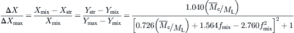 (11.24)
where the coefficients used are as reported by Malkin (1985) which minimize the root mean square error between the predicted thermal performance of a solar water heater with a stratified hot-water storage tank simulated using TRNSYS and that predicted using the f-chart procedure modified for stratified hot-water storage tanks. Equation (11.24) is valid when the value of ![]() is greater than 0.3, which is usual.
is greater than 0.3, which is usual.
The daily average flow through the collector could be estimated from a correlation equivalent to the number of hours (Np) that a solar collector would have a useful energy output. According to Mitchell et al. (1981), for a zero degree differential temperature controller:
![]() (11.25)
(11.25)
![]() = monthly average daily utilizability;
= monthly average daily utilizability;
Ic = critical radiation level (W/m2); and
![]() = solar radiation incident of the collector (kJ/m2 day).
= solar radiation incident of the collector (kJ/m2 day).
It should be noted that by dividing ![]() by 3.6 the units of Np is hours.
by 3.6 the units of Np is hours.
Utilizability is defined as the fraction of the incident solar radiation that can be converted into useful heat by a collector having FR(τα) = 1 and operating at a fixed collector inlet to ambient temperature difference. It should be noted that although the collector has no optical losses and has a heat removal factor of 1, the utilizability is always less than 1 since the collector has thermal losses (see Section 11.2.3). Evans et al. (1982) developed an empirical relationship to calculate the monthly average daily utilizability as a function of the critical radiation level, the monthly average clearness index ![]() given by Eq. (2.82a), the collector tilt angle (β) and the latitude (L):
given by Eq. (2.82a), the collector tilt angle (β) and the latitude (L):
![]() (11.26a)
(11.26a)
where:
![]() (11.26b)
(11.26b)
![]() (11.26c)
(11.26c)
For
![]() (11.27)
(11.27)
where βm is the monthly optimal collector tilt shown in Table 11.10.
Table 11.10
Recommended Monthly Optimal Tilt Angle
| Month | βm (deg.) |
| January | L + 29 |
| February | L + 18 |
| March | L + 3 |
| April | L − 10 |
| May | L − 22 |
| June | L − 25 |
| July | L − 24 |
| August | L − 10 |
| September | L − 2 |
| October | L + 10 |
| November | L + 23 |
| December | L + 30 |
Evans et al. (1982).
Differentiating Eq. (11.26a) and substituting into Eq. (11.25), yields an expression for the monthly average daily collector operating time as:
![]() (11.28)
(11.28)
The monthly average critical radiation level is defined as the level above which useful energy may be collected and is given by:
As can be seen from Eq. (11.29) in order to find the monthly average critical radiation level, a value for the monthly average collector inlet temperature ![]() must be known. This however cannot be determined analytically and it is a function of the thermal stratification in the storage tank. It may be approximated by the Phillip’s stratification coefficient, which is described subsequently. By assuming that the storage tank remains stratified, the monthly average collector inlet temperature may initially be estimated to be the mains water temperature.
must be known. This however cannot be determined analytically and it is a function of the thermal stratification in the storage tank. It may be approximated by the Phillip’s stratification coefficient, which is described subsequently. By assuming that the storage tank remains stratified, the monthly average collector inlet temperature may initially be estimated to be the mains water temperature.
To apply the method an initial estimated value for a flow rate is used and the solar fraction of an active system stratified tank is estimated using the f-chart method by applying the Copsey’s modification for stratified storage. Subsequently, the collector parameters FRUL and FR(τα) are corrected for the estimated flow using Eq. (4.17a). An iterative method is required to determine the “equivalent average” flow rate of a thermosiphon solar water-heating system using the initial estimated value of flow rate (Malkin et al., 1987) as explained subsequently. The average temperature in the storage tank is calculated from a correlation developed between the solar fraction of a thermosiphon system and a non-dimensional form of the monthly average tank temperature obtained from the simulations with TRNSYS indicated above. The least square regression equation obtained is (Malkin et al., 1987):
![]() (11.30)
(11.30)
The average temperature distribution in the system can be predicted from the fraction calculated using the initial estimate of the flow rate allowing an approximate calculation to be made of the thermosiphon head for the system geometry shown in Figure 11.10 (Malkin et al., 1987). This value is then compared to the frictional losses in the collector loop. Iterations need to be made until the agreement between the thermosiphon head and frictional losses are within one percent.
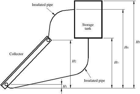
FIGURE 11.10 Thermosiphon system configuration and geometry.
The temperature at the bottom of the storage tank is between the mains temperature (Tm) and the average tank temperature ![]() The proximity of the two temperatures depends on the degree of stratification present. This may be measured approximately using the stratification coefficient, Kstr, defined by Phillips and Dave (1982):
The proximity of the two temperatures depends on the degree of stratification present. This may be measured approximately using the stratification coefficient, Kstr, defined by Phillips and Dave (1982):
![]() (11.31)
(11.31)
The stratification coefficient is also a function of two dimensionless variables; the mixing number, M, and the collector effectiveness, E, given by:
![]() (11.32)
(11.32)
![]() (11.33)
(11.33)
where k is the thermal conductivity of water and H is the storage tank height. Physically, the mixing number is the ratio of conduction to convection heat transfer in the storage tank and in the limit as conduction becomes negligible M approaches zero. Phillips and Dave (1982) showed that:
![]() (11.34)
(11.34)
The temperature of the return fluid from the tank to the collector can be found by solving Eq. (11.31) for Ti. Thus:
![]() (11.35)
(11.35)
Therefore, by using the pump-operating time, estimated from Eq. (11.28), the monthly average temperature of return fluid is approximated as:
![]() (11.36)
(11.36)
It should be noted that if a value is obtained from Eq. (11.36) which is lower than Tm, then Tm is used instead as it is considered impossible to have a storage tank temperature which is lower than the mains temperature.
The collector outlet temperature is found by equating Eq. (3.60), by using It instead of Gt, and an energy balance across the collector:
By integrating Eq. (11.37) on a monthly basis, the monthly average collector fluid outlet temperature can be obtained:
![]() (11.38)
(11.38)
This procedure is undertaken on a monthly basis allowing the “equivalent average” flow rate to be determined and the solar fraction calculated from this value.
Once the monthly average collector fluid inlet and outlet temperatures are known, an estimate of the thermosiphon head may be found based on the relative positions of the tank and the flat-plate collectors as shown in Figure 11.10. Close (1962) has shown that the thermosiphon head generated by the differences in density of fluid in the system may be approximated by making the following assumptions:
1. There are no thermal losses in the connecting pipes.
2. Water from the collector rises to the top of the tank.
3. The temperature distribution in the tank is linear.
Therefore, according to the dimensions indicated in Figure 11.10, the thermosiphon head generated is given by (Close, 1962):
![]() (11.39)
(11.39)
where Si and So are the specific gravities of the fluid at the collector inlet and outlet respectively. Here only direct circulation thermosiphon systems are considered in which water is the collection fluid. The specific gravity according to the temperature (in °C) of water is given by:
![]() (11.40)
(11.40)
The equivalent average flow rate is that which balances the thermosiphon buoyancy force with the frictional resistance in the flow circuit on a monthly average basis. As indicated in Chapter 5 (Section 5.1.1) the flow circuit comprises the collector headers and risers, connecting pipes and storage tank. For each component of the flow circuit, the Darcy–Weisbach equation for friction head loss needs to be employed, given by Eq. (5.6).
The Reynolds number, used to find the type of flow as indicated in Section 5.1.1, at the estimated flow rate is calculated using the following correlation for viscosity as a function of temperature in °C:
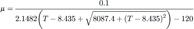 (11.41)
The last term in Eq. (5.6) is included to account for minor friction losses associated with bends, tees, and other restrictions in the piping circuit. It should be noted that although the majority of the pressure drop in the flow circuit occurs across the relatively small diameter collector risers, the minor frictional losses are included to enhance the accuracy of the flow rate estimation. Details of these losses are given in Section 5.1.1 in Chapter 5 and Table 5.2.
All the components of the friction head loss in the flow circuit, at the estimated flow rate, are combined and comparison is made with the previously calculated thermosiphon head. If the thermosiphon head does not balance the frictional losses to within 1% a new guess of the flow rate through the connecting pipes is made by successive substitution. The procedure is repeated with the new estimate of flow rate until the convergence is within 1%.
A new guess of the thermosiphon flow rate can be obtained from (Malkin, 1985):
![]() (11.42)
(11.42)
where subscript p stands for connecting pipes, r for riser, and h for headers.
Convergence is usually obtained by applying no more than three iterations. The resulting single value for monthly average flow rate is that which balances the thermosiphon head with the frictional losses in the flow circuit. As was pointed out before, the solar fraction is calculated, assuming a fixed flow rate operating in an equivalent active system. As in the standard f-chart method, this procedure is carried out for each month of the year, with a previous month’s “equivalent average” flow rate as the initial guess of flow rate for the new month. The fraction of the annual load supplied by solar energy is the sum of the monthly solar energy contributions divided by the annual load as given by Eq. (11.12).
The difference between the TRNSYS simulations and the modified f-chart design method had a reported root mean square error of 2.6% (Malkin, 1985). The procedure is clarified by the following example.
EXAMPLE 11.10
Calculate the solar contribution of a thermosiphon solar water-heating system located in Nicosia, Cyprus for the month of January. The system has the following characteristics:
2. Monthly average solar radiation = 8960 kJ/m2 day (From Appendix 7, Table A7.12)
3. Monthly average ambient temperature = 12.1 °C (From Appendix 7, Table A7.12)
4. Monthly average clearness index = 0.49 (From Appendix 7, Table A7.12)
5. Number of collector panels = 2
6. Collector area per panel = 1.35 m2
7. Collector test FRUL = 21.0 kJ/h m2 °C
9. Collector test flow rate = 71.5 kg/h m2
10. Number of risers per panel = 10
12. Combined header length per panel = 1.9 m
14. Tank-collector connecting pipe length = 2.5 m
15. Collector-tank connecting pipe length = 0.9 m
16. Connecting pipe diameter = 0.022 m
17. Number of bends in connecting pipe = 2
18. Connecting pipe heat-loss coefficient = 10.0 kJ/h m2 °C
19. Storage tank volume = 160 l
21. Storage tank diameter = 0.45 m
22. Daily load draw off = 150 l
23. Mains water temperature = 18 °C
24. Auxiliary set temperature = 60 °C
Solution
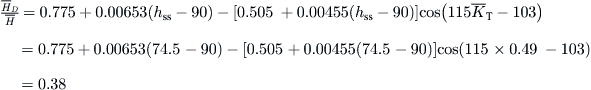
Initially the radiation on the collector surface is required and to save some space the results of Example 11.5 are used. So from Table 11.6 the required value is equal to 14,520 kJ/m2.
An initial estimate of the equivalent average flow rate is 15 kg/h m2 or 40.5 kg/h for a 2.7 m2 collector area. The collector performance parameters FRUL and FR(τα) are corrected for the assumed flow rate, which is different than the test flow rate by using Eq. (5.4b) using the parameter F′UL estimated from Eq. (5.3). Thus:
From Eq. (5.3):

From Eq. (5.4b):
and


Thermal losses from the connecting pipes are estimated from Eq. (5.64b) and Eq. (5.64c):
Therefore:


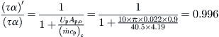
For simplification it is assumed that ![]()
From Eq. (11.21):
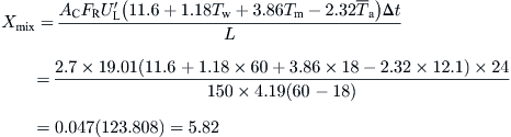
From Eq. (11.22):
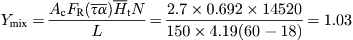
It should be noted that in both the above equations we do not multiply by the number of days in a month as the load is estimated on a daily basis.
Storage capacity = 160/2.7 = 59.3 l/m2, which is different from the standard value of 75 l/m2, so a correction is required estimated from Eq. (11.14): Xmix,c = 5.82 × (59.3/75)−0.25 = 6.17.
From Eq. (11.13): fmix = 1.029Ymix − 0.065Xmix − 0.245Ymix2 + 0.0018Xmix2 + 0.0215Ymix3 = 1.029 × 1.03 − 0.065 × 6.17 − 0.245 × (1.03)2 + 0.0018 × (6.17)2 + 0.0215 × (1.03)3 = 0.49.
To estimate the collector pump operation time a number of parameters are required. From Table 11.10 βm = L + 29° = 35.15 + 29 = 64.15°.
From Eq. (11.27): ![]()
From Eq. (11.26b):
From Eq. (11.26c):
From Eq. (11.29):
From Eq. (11.28):

The ratio ![]() is equal to (8.2 × 40.5)/150 = 2.21.
is equal to (8.2 × 40.5)/150 = 2.21.
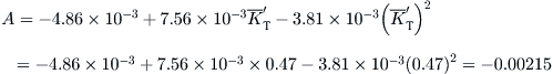
From Eq. (11.24):

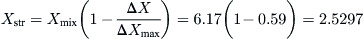
So
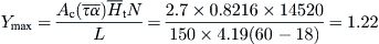
To find ![]() when FR = 1 we solve for FR,high/FR,use at a very high flow rate, say 10,000 kg/h. This gives r = 1.04 and
when FR = 1 we solve for FR,high/FR,use at a very high flow rate, say 10,000 kg/h. This gives r = 1.04 and ![]()
Therefore, from Eq. (11.23):
So from Eq. (11.24):

From Eq. (11.13): fstr = 1.029Ystr − 0.065Xstr − 0.245Ystr2 + 0.0018Xstr2 + 0.0215Ystr3 = 1.029 × 1.1421 − 0.065 × 2.5297 − 0.245 × (1.1421)2 + 0.0018 × (2.5297)2 + 0.0215 × (1.1421)3 = 0.73.
Then the Phillips stratification coefficient is evaluated:
From Eq. (11.32):
From Eq. (11.33):
From Eq. (11.34):

From Eq. (11.30):

Therefore: ![]()
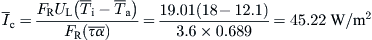
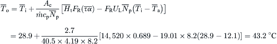
From Eq. (11.36):

Similarly from Eq. (11.38):
Then the specific gravity is estimated from these two temperatures using Eq. (11.40) as:
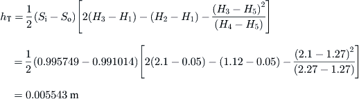
Si = 0.995749 and So = 0.991014. Using the various values of heights and noting that H4 is equal to H5 plus the tank height [=1.27 + 1] in Eq. (11.39):
From Eq. (11.41) using the mean tank temperature: μ = 0.000701 kg/m2 s.
Hydraulic Considerations
The specific gravity of the water in the storage tank, obtained using the mean storage tank temperature in Eq. (11.40) is equal to 0.993439. The mean tank temperature is assumed to flow through the connecting pipes. Therefore, in connecting pipes the velocity is equal to:

which gives: ![]()
Using Eq. (5.7a): f = 64/929 = 0.069. Correcting for developing flow in pipes using Eq. (5.7c):
Therefore f = 0.069 × 1.2141 = 0.084.
Finally, the equivalent pipe length is equal to the actual length of connecting pipes plus the number of bends multiplied by 30 (Table 5.2) multiplied by the pipe diameter = (2.5 + 0.9) + 2 × 30 × 0.022 = 4.72 m. The pipes are of equal diameter so there is no contraction or expansion loss. There is only a loss due to tank entry which is equal to 1 (Table 5.2), so k = 1. Using Eq. (5.6):

Similar calculations for risers give:
Flow rate in risers = 2.025 kg/h
Velocity in risers = 0.0032 m/s
For headers the flow is given by: ![]()
Flow rate in risers = 0.0097 kg/h
Velocity in headers = 0.0096 m/s
Therefore the total friction head Hf is equal to: Hf = 0.000861 + 5.147 × 10⁻⁵ + 0.00012 = 0.00103 m.
By comparing this value with the thermosiphon head estimated before we get a percentage difference of:

As the percentage difference is more than 1% the new flow rate is estimated by Eq. (11.42) which gives 93.8 kg/h.
By repeating this procedure for the new flow rate we get a percentage difference of −29.5%. A new guess of Eq. (11.42) gives a flow rate of 82.4 kg/h which gives a percentage difference of 5.8%. So a third guessing is required which gives a new flow rate equal to 83.7 kg/h which gives:
% difference = 0.04%, which is below 1% so this solution is considered as final. Therefore, the solar contribution at this flow rate is 0.66. This flow rate can also be used as the initial guess for the estimation of the next month’s solar contribution if the estimation is done on an annual basis.
If should be noted that this flow rate is equal to 31 kg/h/m2 [= 83.7 kg/h/2.7 m2] which is about 43% of the test flow rate. Additionally, the number of iterations required depends on how far is the initial guessing of thermosiphonic flow rate from the actual one.
It should be noted that as in earlier examples and due to the large number of calculations required, the use of a spreadsheet program greatly facilitates the calculations, especially at the iteration stage.
11.1.5 General remarks
The f-chart design method is used to quickly estimate the long-term performance of solar energy systems of standard configurations. The input data needed are the monthly average radiation and temperature, the monthly load required to heat a building and its service water, and the collector performance parameters obtained from standard collector tests. A number of assumptions are made for the development of the f-chart method. The main ones include assumptions that the systems are well built, system configuration and control are close to the ones considered in the development of the method, and the flow rate in the collectors is uniform. If a system under investigation differs considerably from these conditions, then the f-chart method cannot give reliable results.
It should be emphasized that the f-chart is intended to be used as a design tool for residential space and domestic water-heating systems of standard configuration. In these systems, the minimum temperature at the load is near 20 °C; therefore, energy above this value of temperature is useful. The f-chart method cannot be used for the design of systems that require minimum temperatures substantially different from this minimum value. Therefore, it cannot be used for solar air conditioning systems using absorption chillers, for which the minimum load temperature is around 80 °C.
It should also be understood that, because of the nature of the input data used in the f-chart method, there are a number of uncertainties in the results obtained. The first uncertainty is related to the meteorological data used, especially when horizontal radiation data are converted into radiation falling on the inclined collector surface, because average data are used, which may differ considerably from the real values of a particular year, and that all days were considered symmetrical about a solar noon. A second uncertainty is related to the fact that solar energy systems are assumed to be well built with well-insulated storage tanks and no leaks in the system, which is not very correct for air systems, all of which leak to some extent, leading to a degraded performance. Additionally, all liquid storage tanks are assumed to be fully mixed, which leads to conservative long-term performance predictions because it gives overestimation of collector inlet temperature. The final uncertainty is related to the building and hot water loads, which strongly depend on variable weather conditions and the habits of the occupants.
Despite these limitations, the f-chart method is a handy method that can easily and quickly be used for the design of residential-type solar heating systems. When the main assumptions are fulfilled, quite accurate results are obtained.
11.1.6 f-chart program
Although the f-chart method is simple in concept, the required calculations are tedious, particularly for the manipulation of radiation data. The use of computers greatly reduces the effort required. Program f-chart (Klein and Beckman, 2005), developed by the originators of TRNSYS, is very easy to use and gives predictions very quickly. Again, in this case, the model is accurate only for solar heating systems of a type comparable to that which was assumed in the development of the f-chart.
The f-chart program is written in the BASIC programming language and can be used to estimate the long-term performance of solar energy systems that have flat-plate, evacuated tube collectors, compound parabolic collectors, and one- or two-axis tracking concentrating collectors. Additionally, the program includes an active–passive storage system and analyzes the performance of a solar energy system in which energy is stored in the building structure rather than a storage unit (treated with methods presented in the following section) and a swimming pool-heating system that provides estimates of the energy losses from the swimming pool. The complete list of solar energy systems that can be handled by the program is as follows:
• Pebble-bed storage space and domestic water heating systems.
• Water-storage space and/or domestic water heating systems.
• Active collection with building storage space-heating systems.
• Direct gain passive systems.
• Collector-storage wall passive systems.
• General heating systems, such as process heating systems.
• Integral collector-storage domestic water-heating systems.
The program can also perform economic analysis of the systems. The program, however, does not provide the flexibility of detailed simulations and performance investigations, as TRNSYS does.
Leave a Reply