
The electrical power output from a PV panel depends on the incident radiation, the cell temperature, the solar incidence angle, and the load resistance. In this section, a method to design a PV system is presented and all these parameters are analyzed. Initially, a method to estimate the electrical load of an application is presented, followed by the estimation of the absorbed solar radiation from a PV panel and a description of the method for sizing PV systems.
9.5.1 Electrical loads
As is already indicated, a PV system size may vary from a few watts to hundreds of kilowatts. In grid-connected systems, the installed power is not so important because the produced power, if not consumed, is fed into the grid. In stand-alone systems, however, the only source of electrical power is the PV system; therefore, it is very important at the initial stages of the system design to assess the electrical loads the system will cover. This is especially important in emergency warning systems. The main considerations that a PV system designer needs to address from the very beginning are:
1. According to the type of loads that the PV system will meet, which is more important, the total daily energy output or the average or peak power?
2. At what voltage will the power be delivered, and is it AC or DC?
3. Is a backup energy source needed?
Usually the first things the designer has to estimate are the load and the load profile that the PV system will meet. It is very important to be able to estimate precisely the loads and their profiles (time when each load occurs). Due to the initial expenditure needed, the system is sized at the minimum required to satisfy the specific demand. If, for example, three appliances exist, requiring 500 W, 1000 W, and 1500 W, respectively; each appliance is to operate for 1 h; and only one appliance is on at a time, then the PV system must have an installed peak power of 1500 W and 3000 Wh of energy requirement. If possible, when using a PV system, the loads should be intentionally spread over a period of time to keep the system small and thus cost-effective. Generally, the peak power is estimated by the value of the highest power occurring at any particular time, whereas the energy requirement is obtained by multiplying the wattage of each appliance by the operating hours and summing the energy requirements of all appliances connected to the PV system. The maximum power can easily be estimated with the use of a time-schedule diagram, as shown in the following example.
EXAMPLE 9.4
Estimate the daily load and the peak power required by a PV system that has three appliances connected to it with the following characteristics:
1. Appliance 1, 20 W operated for 3 h (10 am–1 pm).
2. Appliance 2, 10 W operated for 8 h (9 am–5 pm).
3. Appliance 3, 30 W operated for 2 h (2 pm–4 pm).
Solution
The daily energy use is equal to:

To find the peak power, a time schedule diagram is required (see Figure 9.20).
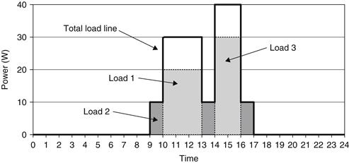
FIGURE 9.20 Time schedule diagram.
As can be seen, the peak power is equal to 40 W.
EXAMPLE 9.5
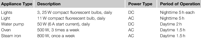
A remote cottage has the loads listed in Table 9.2. Find the average load and peak power to be satisfied by a 12 V PV system with an inverter.
Table 9.2
Loads for Cottage in Example 9.5
Solution
In Table 9.3, the loads for this application are separated according to type of power. Because no information is given about the time schedule of the loads, these are assumed to occur simultaneously.
Table 9.3
Loads in Table 9.2, by Type of Power
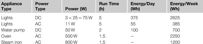
From Table 9.3, the following can be determined:


9.5.2 Absorbed solar radiation
The main factor affecting the power output from a PV system is the absorbed solar radiation, S, on the PV surface. As was seen in Chapter 3, S depends on the incident radiation, air mass, and incident angle. As in the case of thermal collectors, when radiation data on the plane of the PV are unknown, it is necessary to estimate the absorbed solar radiation using the horizontal data and information on incidence angle. As in thermal collectors, the absorbed solar radiation includes the beam, diffuse, and ground-reflected components. In the case of PVs, however, a spectral effect is also included. Therefore, by assuming that the diffuse and ground-reflected radiation is isotropic, S can be obtained from (Duffie and Beckman, 2006):
![]() (9.25)
(9.25)
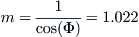
where M = air mass modifier.
The air mass modifier, M, accounts for the absorption of radiation by species in the atmosphere, which causes the spectral content of the available solar radiation to change, thus altering the spectral distribution of the incident radiation and the generated electricity. An empirical relation that accounts for the changes in the spectral distribution resulting from changes in the air mass, m, from the reference air mass of 1.5 (at sea level) is given by the following empirical relation developed by King et al. (2004):
![]() (9.26)
(9.26)
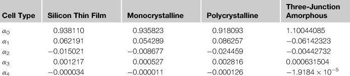
Constant αi values in Eq. (9.26) depend on the PV material, although for small zenith angles, less than about 70°, the differences are small (De Soto et al., 2006). Table 9.4 gives the values of the αi constants for various PV panels tested at the National Institute of Standards and Technology (NIST) (Fanney et al., 2002).
Table 9.4
Values of αi Constants for Various PV Panels Tested at NIST
As was seen in Chapter 2, Section 2.3.6, the air mass, m, is the ratio of the mass of air that the beam radiation has to traverse at any given time and location to the mass of air that the beam radiation would traverse if the sun were directly overhead. This can be given from Eq. (2.81) or from the following relation developed by King et al. (1998):
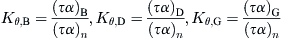
As the incidence angle increases, the amount of radiation reflected from the PV cover increases. Significant effects of inclination occur at incidence angles greater than 65°. The effect of reflection and absorption as a function of incidence angle is expressed in terms of the incidence angle modifier, Kθ, defined as the ratio of the radiation absorbed by the cell at incidence angle θ divided by the radiation absorbed by the cell at normal incidence. Therefore, in equation form, the incidence angle modifier at angle θ is obtained by:
![]() (9.28)
(9.28)
It should be noted that the incidence angle depends on the PV panel slope, location, and time of the day. As in thermal collectors, separate incidence angle modifiers are required for the beam, diffuse, and ground-reflected radiation. For the diffuse and ground-reflected radiation, the effective incidence angle given by Eq. (3.4) can be used. Although these equations were obtained for thermal collectors, they were found to give reasonable results for PV systems as well.
So, using the concept of incidence angle modifier and noting that:
Equation (9.25) can be written as:
![]() (9.29)
(9.29)
It should be noted that, because the glazing is bonded to the cell surface, the incidence angle modifier of a PV panel differs slightly from that of a flat-plate collector and is obtained by combining the various equations presented in Chapter 2, Section 2.3.3:
![]() (9.30)
(9.30)
where θ and θr are the incidence angle and refraction angle (same as angles θ1 and θ2 in Section 2.3.3). A typical value of the extinction coefficient, K, for PV systems is 4m-1 (for water white glass), glazing thickness is 2 mm, and the refractive index for glass is 1.526.
A simpler way to obtain the incidence angle modifier is given by King et al. (1998), who suggested the following equation:
![]() (9.31)
(9.31)
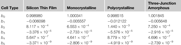
Table 9.5 gives the values of the bi constants for various PV panels tested at NIST (Fanney et al., 2002).
Table 9.5
Values of bi Constants for Various PV Panels Tested at NIST
Therefore, Eq. (9.31) can be used directly for the specific type of cell to give the incidence angle modifier according to the incidence angle. Again, for the diffuse and ground-reflected radiation, the effective incidence angle given by Eq. (3.4) can be used.
EXAMPLE 9.6
A south-facing PV panel is installed at 30° in a location which is at 35°N latitude. If, on June 11 at noon, the beam radiation is 715 W/m2 and the diffuse radiation is 295 W/m2, both on a horizontal surface, estimate the absorbed solar radiation on the PV panel. The thickness of the glass cover on PV is 2 mm, the extinction coefficient K is 4m−1, and ground reflectance is 0.2.
Solution
From Table 2.1, on June 11, δ = 23.09°. First, the effective incidence angles need to be calculated. For the beam radiation, the incidence angle is required, estimated from Eq. (2.20):

For the diffuse and ground-reflected components, Eq. (3.4) can be used:


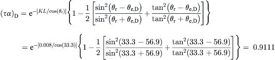
Next, we need to estimate the three incidence angle modifiers. At an incidence angle of 18.1°, the refraction angle from Eq. (2.44) is:

Using Eq. (9.30) with K = 4m−1 and L = 0.002 m,

At normal incidence, as shown in Chapter 2, Section 2.3.3, Eq. (2.49), the term in the square bracket of Eq. (9.30) is replaced with 1 − [(n − 1)/(n + 1)]2. Therefore,
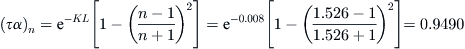
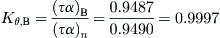
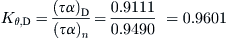
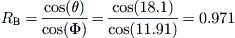
And from Eq. (9.28),
For the diffuse radiation,

Using Eq. (9.30),
And from Eq. (9.28),
Using Eq. (9.31) for monocrystalline cells gives Kθ,D = 0.9622; and for polycrystalline cells, Kθ,D = 0.9672. Both values are close to the value just obtained, so even if the exact type of PV cell is not known, acceptable values can be obtained from Eq. (9.31) using either type of the cell.
For the ground-reflected radiation,

Using Eq. (9.30),
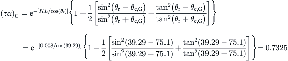
And from Eq. (9.28),
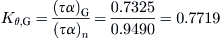
Using Eq. (9.31) for monocrystalline cells gives Kθ,G = 0.7625, and for polycrystalline cells, Kθ,G = 0.7665. Both values, again, are close to the value obtained previously.
For the estimation of the air mass, the zenith angle is required, obtained from Eq. (2.12):

The air mass is obtained from Eq. (9.27):

It should be noted that the same result is obtained using Eq. (2.81):
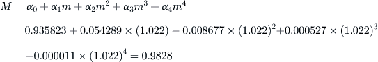
From Eq. (9.26),
From Eq. (2.88),
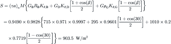
Now, using Eq. (9.29),
9.5.3 Cell temperature
As was seen in Section 9.1.3, the performance of the solar cell depends on the cell temperature. This temperature can be determined by an energy balance and considering that the absorbed solar energy that is not converted to electricity is converted to heat, which is dissipated to the environment. Generally, when operating solar cells at elevated temperatures, their efficiency is lowered. In cases where this heat dissipation is not possible, as in BIPVs and concentrating PV systems (see Section 9.7), the heat must be removed by some mechanical means, such as forced air circulation, or by a water heat exchanger in contact with the back side of the PV. In this case, the heat can be used to an advantage, as explained in Section 9.8; these systems are called hybrid photovoltaic/thermal (PV/T) systems. Because these systems offer a number of advantages, even normal roof-mounted PVs can be converted into hybrid PV/Ts.
The energy balance on a unit area of a PV module that is cooled by heat dissipation to ambient air is given by:
![]() (9.32)
(9.32)
For the (τα) product, a value of 0.9 can be used without serious error (Duffie and Beckman, 2006). The heat loss coefficient, UL, includes losses by convection and radiation from the front and back of the PV to the ambient temperature, Ta.
By operating the module at the nominal operating cell temperature (NOCT) conditions (see Table 9.1) with no load, i.e. ηe = 0, Eq. (9.32) becomes:
![]() (9.33)
(9.33)
which can be used to determine the ratio:
![]() (9.34)
(9.34)
By substituting Eq. (9.34) into Eq. (9.32) and performing the necessary manipulations, the following relation can be obtained:
An empirical formula that can be used for the calculation of PV module temperature of polycrystalline silicon solar cells was presented by Lasnier and Ang (1990). This is a function of the ambient temperature, Ta, and the incoming solar radiation, Gt, given by:
![]() (9.36)
(9.36)
When the temperature coefficient of the PV module is given, the following equation can be used to estimate the efficiency according to the cell temperature:
![]() (9.37)
(9.37)
β = temperature coefficient (per k−1).
EXAMPLE 9.7
If, for a PV module operating at NOCT conditions, the cell temperature is 42 °C, determine the cell temperature when this module operates at a location where Gt = 683 W/m2, V = 1 m/s, and Ta = 41 °C and the module is operating at its maximum power point with an efficiency of 9.5%.
Solution
Using Eq. (9.35),

Using empirical Eq. (9.36),

As can be seen, the empirical method is not as accurate but offers a good approximation.
It should be noted that, in Example 9.7, the module efficiency was given. If it was not given, then a trial-and-error solution needs to be applied. In this procedure, a value of module efficiency is assumed and TC is estimated using Eq. (9.35). Provided that Io and Isc are known, the value of TC is used to find Vmax with Eq. (9.14). Subsequently, Pmax and ηmax are estimated with Eqs (9.17) and (9.18), respectively. The initial guess value of ηe is then compared with ηmax, and if there is a difference, iteration is used. Because the efficiency is strongly related to cell temperature, fast convergence is achieved.
9.5.4 Sizing of PV systems
Once the load and absorbed solar radiation are known, the design of the PV system can be carried out, including the estimation of the required PV panel’s area and the selection of the other equipment, such as controllers and inverters. Detailed simulations of PV systems can be carried with the TRNSYS program (see Chapter 11, Section 11.5.1); however, usually a simple procedure needs to be followed to perform a preliminary sizing of the system. The simplicity of this preliminary design depends on the type of the application. For example, a situation in which a vaccine refrigerator is powered by the PV system, and a possible failure of the system to supply the required energy will destroy the vaccines is much different to a home system delivering electricity to a television and some lamps.
The energy delivered by a PV array, EPV, is given by:
![]() (9.38)
(9.38)
![]() = monthly average value of Gt, obtained from Eq. (2.97) by setting all parameters as monthly average values.
= monthly average value of Gt, obtained from Eq. (2.97) by setting all parameters as monthly average values.
A = area of the PV array (m2).
The energy of the array available to the load and battery, EA, is obtained from Eq. (9.38) by accounting for the array losses, LPV, and other power conditioning losses, LC:
![]() (9.39)
(9.39)
Therefore, the array efficiency is defined as:
![]() (9.40)
(9.40)
Grid-connected systems
The inverter size required for grid-connected systems is equal to the nominal array power. The energy available to the grid is simply what is produced by the array multiplied by the inverter efficiency:
![]() (9.41)
(9.41)
Usually, some distribution losses are present accounted by ηdist and, if not, all this energy can be absorbed by the grid, then the actual energy delivered, Ed, is obtained by accounting for the grid absorption rate, ηabs, from:
![]() (9.42)
(9.42)
Stand-alone systems
For stand-alone systems, the total equivalent DC demand, Ddc,eq, is obtained by summing the total DC demand, Ddc, and the total AC demand, Dac (both expressed in kilowatt hours per day), converted to DC equivalent using:
![]() (9.43)
(9.43)
When the array supplies all energy to a DC load, the actual energy delivered, Ed,dc, is obtained by:
![]() (9.44)
(9.44)
When the battery directly supplies a DC load, the efficiency of the battery, ηbat, is accounted for, and the actual energy delivered, Ed,dc,bat, is obtained from:
![]() (9.45)
(9.45)
When the battery is used to supply energy to an AC load, the inverter efficiency is also accounted for:
![]() (9.46)
(9.46)
Finally, when the array supplies all energy to an AC load, the actual energy delivered, Ed,ac, is obtained by:
![]() (9.47)
(9.47)
This methodology is demonstrated by means of two examples. The first is a simple one and the second takes into account the various efficiencies.
EXAMPLE 9.8
A PV system is using 80 W, 12 V panels and 6 V, 155 Ah batteries in a good sunshine area. The battery efficiency is 73% and the depth of discharge is 70%. If, in wintertime, there are 5 h of daylight, estimate the number of PV panels and batteries required for a 24 V application with a load of 2600 Wh.
Solution
The number of PV panels required is obtained from:

Because the system voltage is 24 V and each panel produces 12 V, two panels need to be connected in series to produce the required voltage, so an even number is required; therefore, the number of PV panels is increased to eight.
If, for the location with good sunshine, we consider that three days of storage would be adequate, the storage required is:

Again as the system voltage is 24 V and each battery is 6 V, we need to connect 4 batteries in series, so the number of batteries to use here is either 16 (very close to 16.4, with the possibility of not having enough power for the third day) or 20 (for more safety).
The second example uses the concept of efficiency of the various components of the PV system.
EXAMPLE 9.9
Using the data from Example 9.5, estimate the expected daily energy requirement. The efficiencies of the various components of the system are:
Solution
From Example 9.5, the average DC load was 475 Wh and the average AC load was 547.9 Wh. These give a total load of 1022.9 Wh.
Expected daily loads are (from Example 9.5):
• Day DC = 100 Wh (from PV system).
• Night DC = 375 Wh (from battery).
• Night AC = 55 Wh (from battery).
• Day AC = 492.9 Wh, = (2250 + 1200)/7 (from PV system through the inverter).
The various energy requirements are obtained as follows:
• Day DC energy is obtained from Eq. (9.44): Ed,dc = EAηdist, so EA = 100/0.95 = 105.3 Wh.
• Night DC energy is obtained from Eq. (9.45): Ed,dc,bat = EAηbatηdist, so EA = 375/(0.75 × 0.95) = 526.3 Wh.
• Night AC energy is obtained from Eq. (9.46): Ed,ac,bat = EAηbatηinvηdist, so EA = 55/(0.75 × 0.90 × 0.95) = 85.8 Wh.
• Day AC energy is obtained from Eq. (9.47): Ed,ac = EAηinvηdist, so, EA = 492.9/(0.90 × 0.95) = 576.5 Wh.
• Expected daily energy requirement = 105.3 + 526.3 + 85.8 + 576.5 = 1293.9 Wh.
Therefore the energy requirement is increased by 27% compared to 1022.9 Wh estimated before.
One way utilities historically have thought about generation reliability is loss-of-load probability (LLP). LLP is the probability that a generation will be insufficient to meet demand at some point over some specific time window, and this principle can also be used in sizing stand-alone PV systems. Therefore, the merit of a stand-alone PV system should be judged in terms of the reliability of the electricity supply to the load. Specifically, for stand-alone PV systems, LLP is defined as the ratio between the energy deficit and the energy demands both on the load and over a long period of time. Because of the random nature of the solar radiation, the LLP of even a trouble-free PV system is always greater than 0.
Any PV system consists mainly of two subsystems that need to be designed: the PV array (also called the generator) and the battery storage system (also called the accumulator). A useful definition of these parameters relates to the load. Therefore, on a daily basis, the PV array capacity, CA, is defined as the ratio between the mean PV array energy production and the mean load energy demand. The storage capacity, CS, is defined as the maximum energy that can be taken out from the accumulator divided by the mean load energy demand. According to Egido and Lorenzo (1992), the sizing pair CA and CS can be given by the following equations:
![]() (9.48)
(9.48)
![]() (9.49)
(9.49)
Ht = mean daily irradiation on the PV array (Wh/m2).
L = mean daily energy consumption (Wh).
C = useful accumulator capacity (Wh).
The reliability of a PV system is defined as the percentage of load satisfied by the PV system, whereas the LLP is the percentage of the mean load (over large periods of time) not supplied by the PV system, i.e., it is the opposite of reliability.
As can be understood from Eqs (9.48) and (9.49), it is possible to find many different combinations of CA and CS leading to the same LLP value. However, the larger the PV system size, the greater is the cost and the lower the LLP. Therefore, the task of sizing a PV system consists of finding the better trade-off between cost and reliability. Very often, the reliability is an a priori requirement from the user, and the problem is to find the pair of CA and CS values that lead to a given LLP value at the minimum cost.
Additionally, because CA depends on the meteorological conditions of the location, this means that the same PV array for the same load can be “large” in one site and “small” in another site with lower solar radiation.
In cases where long-term averages of daily irradiation are available in terms of monthly means, Eq. (9.48) is modified as:
![]() (9.50)
(9.50)
where ![]() = monthly average daily irradiation on the PV array (Wh/m2).
= monthly average daily irradiation on the PV array (Wh/m2).
In this case,![]() is defined as the ratio of the average energy output of the generator in the month with worst solar radiation input divided by the average consumption of the load (assuming a constant consumption of load for every month).
is defined as the ratio of the average energy output of the generator in the month with worst solar radiation input divided by the average consumption of the load (assuming a constant consumption of load for every month).
Each point of the CA–CS plane represents a size of a PV system. This allows one to map the reliability, as is shown in Figure 9.21. The curve is the loci of all the points corresponding to a same LLP value. Because of that, this type of curve is called an iso-reliability curve. In Figure 9.21, an example LLP curve is represented for LLP equal to 0.01.
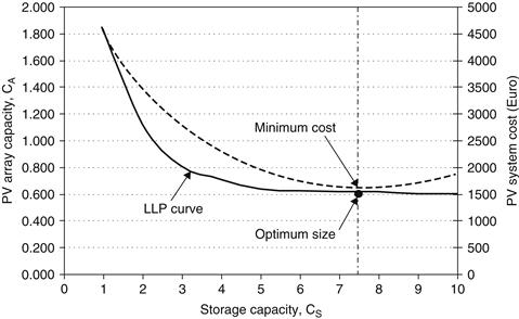
FIGURE 9.21 LLP curve for LLP = 0.01 and cost curve of a PV system.
It should be noted that the definitions of CA and CS imply that this map is independent of the load and depends only on the meteorological behavior of the location. As can be seen from Figure 9.21, the iso-reliability curve is very nearly a hyperbola with its asymptotes parallel to the x and y axes, respectively. For a given LLP value, the plot of the cost of the PV systems (dashed line in Figure 9.21) corresponding to the iso-reliability curve is, approximately, a parabola having a minimum that defines the optimal solution to the sizing problem.
The LLP curve represents pairs of CS and CA values that lead to the same value of LLP. This means, for example, that for the pair (CS, CA) = (2, 1.1), the proposed reliability is achieved by having a “big” generator and a “small” storage system. Similarly, for the same reliability, the pair (CS, CA) = (9, 0.6) leads to a “small” generator and a “big” battery. As can be seen, the optimum size of the system is at (CS, CA) = (7.5, 0.62), which gives the minimum PV system cost.
Many methods have been developed by researchers to establish relations between CA, CS, and LLP. The main ones are numerical methods that use detailed system simulations and analytical methods that use equations describing the behavior of the PV system. These methods are presented by Egido and Lorenzo (1992).
Fragaki and Markvart (2008) developed a new sizing approach applied to stand-alone PV systems design, based on system configurations without shedding load. The investigation is based on a detailed study of the minimum storage requirement and an analysis of the sizing curves. The analysis revealed the importance of using daily series of measured solar radiation data instead of monthly average values. Markvart et al. (2006) presented the system sizing curve as superposition of contributions from individual climatic cycles of low daily solar radiation for a location southeast of England.
Hontoria et al. (2005) used an artificial neural network (ANN) (see Chapter 11) to generate the sizing curve of stand-alone PV systems from CS, LLP, and daily clearness index. Mellit et al. (2005) also used an ANN architecture for estimating the sizing coefficients of stand-alone PV systems based on the synthetic and measured solar radiation data.
Once the LLP curves are obtained, it is very simple to design both the capacity of the generator (CA) and the accumulator capacity (CS). Depending on the reliability needed for the PV system design, a specific value of the LLP is considered. For instance, Table 9.6 shows some usual values for typical PV systems.
Table 9.6
Recommended LLP Values for Various Applications
| Application | LLP |
| Domestic appliances | 10−1 |
| Rural home lighting | 10−2 |
| Telecommunications | 10−4 |
Leave a Reply