
In this chapter so far, we have seen simple methods that can be used to design active solar energy systems of standard configuration using f-chart and other solar processes with the utilizability methods. Although these methods are proven to be accurate enough and possible to carry out with hand calculations, the most accurate way to estimate the performance of solar processes is with detailed simulation.
The proper sizing of the components of a solar energy system is a complex problem that includes both predictable (collector and other performance characteristics) and unpredictable (weather data) components. The initial step in modeling a system is the derivation of a structure to be used to represent the system. It will become apparent that there is no unique way of representing a given system. Since the way the system is represented often strongly suggests specific modeling approaches, the possibility of using alternative system structures should be left open while the modeling approach selection is being made. The structure that represents the system should not be confused with the real system. The structure will always be an imperfect copy of reality. However, the act of developing a system structure and the structure itself will foster an understanding of the real system. In developing a structure to represent a system, system boundaries consistent with the problem being analyzed are first established. This is accomplished by specifying what items, processes, and effects are internal to the system and what items, processes, and effects are external.
Simplified analysis methods have the advantages of computational speed, low cost, rapid turnaround (which is especially important during iterative design phases), and ease of use by persons with little technical experience. The disadvantages include limited flexibility for design optimization, lack of control over assumptions, and a limited selection of systems that can be analyzed. Therefore, if the system application, configuration, or load characteristics under consideration are significantly non-standard, a detailed computer simulation may be required to achieve accurate results.
Computer modeling of thermal systems presents many advantages, the most important of which are the following:
1. They eliminate the expense of building prototypes.
2. Complex systems are organized in an understandable format.
3. They provide a thorough understanding of the system operation and component interactions.
4. It is possible to optimize the system components.
5. They estimate the amount of energy delivery from the system.
6. They provide temperature variations of the system.
7. They estimate the design variable changes on system performance by using the same weather conditions.
Simulations can provide valuable information on the long-term performance of solar energy systems and the system dynamics. This includes temperature variations, which may reach to values above the degradability limit (e.g., for selective coatings of collector absorber plates) and water boiling, with consequent heat dumping through the relief valve. Usually, the detail or type of output obtained by a program is specified by the user; the more detailed the output required, the more intensive are the calculations, which leads to extended computer time required to obtain the results.
Over the years a number of programs have been developed for the modeling and simulation of solar energy systems. Some of the most popular ones are described briefly in this section. These are the well-known programs TRNSYS, WATSUN, and Polysun. The chapter concludes with a brief description of artificial intelligence techniques used recently for the modeling and performance evaluation of solar and other energy systems.
11.5.1 TRNSYS simulation program
TRNSYS is an acronym for “transient simulation”, which is a quasi-steady simulation model. This program, currently in version 17.1 (Klein et al., 2010), was developed at the University of Wisconsin by the members of the Solar Energy Laboratory and written in the FORTRAN computer language. The first version was developed in 1977 and, so far, has undergone 12 major revisions. The program was originally developed for use in solar energy applications, but the use was extended to include a large variety of thermal and other processes, such as hydrogen production, photovoltaics (PVs), and many more. The program consists of many subroutines that model subsystem components. The mathematical models for the subsystem components are given in terms of their ordinary differential or algebraic equations. With a program such as TRNSYS, which can interconnect system components in any desired manner, solve differential equations, and facilitate information output, the entire problem of system simulation reduces to a problem of identifying all the components that make up the particular system and formulating a general mathematical description of each (Kalogirou, 2004b). The users can also create their own programs, which are no longer required to be recompiled with all other program subroutines but just as a dynamic link library (DLL) file with any FORTRAN compiler and put in a specified directory.
Simulations generally require some components that are not ordinarily considered as part of the system. Such components are utility subroutines and output-producing devices. The TYPE number of a component relates the component to a subroutine that models that component. Each component has a unique TYPE number. The UNIT number is used to identify each component (which can be used more than once). Although two or more system components can have the same TYPE number, each must have a unique UNIT number. Once all the components of the system have been identified and a mathematical description of each component is available, it is necessary to construct an information flow diagram for the system. The purpose of the information flow diagram is to facilitate identification of the components and the flow of information between them. Each component is represented as a box, which requires a number of constant PARAMETERS and time-dependent INPUTS and produces time-dependent OUTPUTS. An information flow diagram shows the manner in which all system components are interconnected. A given OUTPUT may be used as an INPUT to any number of other components. From the flow diagram, a deck file has to be constructed, containing information on all components of the system, the weather data file, and the output format.
Subsystem components in the TRNSYS include solar collectors, differential controllers, pumps, auxiliary heaters, heating and cooling loads, thermostats, pebble bed storage, relief valves, hot-water cylinders, heat pumps, and many more. Some of the main ones are shown in Table 11.17. There are also subroutines for processing radiation data, performing integrations, and handling input and output. Time steps down to 1/1000 h (3.6 s) can be used for reading weather data, which makes the program very flexible with respect to using measured data in simulations. Simulation time steps at a fraction of an hour are also possible.
Table 11.17
Main Components in the Standard Library of TRNSYS 17
| Building Loads and Structures | Hydronics |
| Energy/degree-hour house | Pump |
| Roof and attic | Fan |
| Detailed zone | Pipe |
| Overhang and wingwall shading | Duct |
| Thermal storage wall | Various fittings (tee-piece, diverter, tempering valve) |
| Attached sunspace | Pressure relief valve |
| Detailed multi-zone building | Output Devices |
| Controller Components | Printer |
| Differential controllers | Online plotter |
| Three-stage room thermostat | Histogram plotter |
| PID controller | Simulation summary |
| Microprocessor controller | Economics |
| Collectors | Physical Phenomena |
| Flat-plate collector | Solar radiation processor |
| Performance map solar collector | Collector array shading |
| Theoretical flat-plate collector | Psychrometrics |
| Thermosiphon collector with integral storage | Weather-data generator |
| Evacuated tube solar collector | Refrigerant properties |
| Compound parabolic collector | Undisturbed ground-temperature profile |
| Electrical Components | Thermal Storage |
| Regulators and inverters | Stratified fluid storage tank |
| Photovoltaic array | Rock-bed thermal storage |
| Photovoltaic-thermal collector | Algebraic tank |
| Wind-energy conversion system | Variable volume tank |
| Diesel engine generator set | Detailed storage tank |
| Power conditioning | Utility Components |
| Lead-acid battery | Data file reader |
| Heat Exchangers | Time-dependent forcing function |
| Constant effectiveness heat exchanger | Quantity integrator |
| Counter flow heat exchanger | Calling Excell |
| Cross-flow heat exchanger | Calling EES |
| Parallel-flow heat exchanger | Calling CONTAM |
| Shell and tube heat exchanger | Calling MATLAB |
| Waste heat recovery | Calling COMIS |
| HVAC Equipment | Holiday calculator |
| Auxiliary heater | Input value recall |
| Dual source heat pump | Weather-Data Reading |
| Cooling towers | Standard format files |
| Single-effect hot water-fired absorption chiller | User format files |
In addition to the main TRNSYS components, an engineering consulting company specializing in the modeling and analysis of innovative energy systems and buildings, Thermal Energy System Specialists (TESS), developed libraries of components for use in TRNSYS. Currently, the TESS library includes more than 500 TRNSYS components. Each of the component libraries comes with a TRNSYS Model File (∗.tmf) to use in the Simulation Studio interface, source code, and an example TRNSYS Project (∗.tpf) that demonstrates typical uses of the component models found in that library. With the release of the TESS Libraries version 17.0 (numbering system changed to be compatible with TRNSYS version number), over 90 new models with many new examples have been added from the previous version 2.0. According to TRNSYS website (www.trnsys.com/tess-libraries/) TESS Component Libraries for TRNSYS 17 fall into 14 categories as follows:
1. Application Components. This is an assortment of scheduling and setpoint applications that use the TRNSYS Simulation Studio plug-in feature and are useful for creating daily, weekly, monthly schedules, normalized occupancy, lighting, or equipment schedules and setpoints for thermostats.
2. Controller Components. This includes numerous controllers, which can be used in practically any TRNSYS simulation and range from a simple thermostat controller to a complex multi-stage differential controller with minimum on and off times and from a tempering valve controller to an outside air-reset controller.
3. Electrical Components. This includes components for solar PV and combined solar thermal (PV/T) modeling in TRNSYS and also building integrated PV models, a PV array shading component, an equipment outage component, and lighting controls.
4. Geothermal Heat Pump (GHP) Components. This includes not only extensive ground heat exchanger models (horizontal multi-layer ground heat exchanger and the vertical heat exchanger), but also buried single and double pipes, and various heat pump models.
5. Ground Coupling Components. This includes components to compute the energy transfer between an object (building slabs, basements, buried thermal storage tanks, etc.) and the surrounding ground.
6. HVAC Equipment Components. This library contains more than 60 different components for modeling anything related to heating, ventilation, and air conditioning of buildings as well as residential, commercial, and industrial HVAC components.
7. Hydronic Components. This contains components for a variety of fans, pumps, valves, plenums, duct and pipe components that are essential for working with fluid loops in a TRNSYS simulation.
8. Loads and Structures Components. This library contains alternatives to the standard TRNSYS building model components and includes a synthetic building (load-curve generator), a simple multi-zone building and methods for imposing pre-calculated building loads (generated not only by TRNSYS but also by other software) onto a TRNSYS system or plant simulation.
9. Optimization Components. This is also known as TRNOPT, which is a tool that couples the TRNSYS simulation with GenOpt program for the minimization of a cost or error function (see Section 11.6.2). TRNOPT may also be used to calibrate simulation results to the data from the actual system.
10. Solar Collector Components. This contains 18 different solar collector components varying from different theoretical and test-based collectors to collectors with different glazings.
11. Storage Tank Components. This contains in addition to the standard vertical cylindrical storage tank, spherical, rectangular and horizontal cylindrical tank models. It includes also a wrap-around heat exchanger tank, aquastats, a heat pump water heater and a zip water heater.
12. Utility Components. This is a collection of useful components for TRNSYS simulations including random number generators, water draw profiles, an “event triggered” printer, a wind speed calculator, an economics routine, building infiltration models, and many more.
13. Combined Heat and Power (CHP) Components. This includes many steam system components such as pumps, valves, superheaters, de-superheaters, turbines, etc., which can be used to simulate different cogeneration or trigeneration systems at different scales.
14. High-Temperature Solar Components. This contains components that have temperature-dependent thermo-physical fluid properties such as a parabolic trough collector, valves, pumps, expansion tanks, and pipes. These properties concern mainly the specific heat of the collector’s working fluid, which although for low temperature applications can be considered as constant, this is not appropriate for high temperature collectors or for the heat transfer fluids typically employed by these collectors.
Another interesting application developed for TRNSYS is the library for Solar Thermal Electric Components (STEC). This library includes the necessary components, which can be used for modeling and simulation of Concentrating Solar Power (CSP) systems and comprises models for thermodynamic properties, Brayton and Rankine Cycles, solar thermal electric and storage sub-libraries.
Model validation studies have been conducted to determine the degree to which the TRNSYS program serves as a valid simulation program for a physical system. The use of TRNSYS for the modeling of a thermosiphon solar water heater was also validated by the author and found to be accurate within 4.7% (Kalogirou and Papamarcou, 2000).
TRNSYS used to be a non-user-friendly program; the latest versions of the program (version 16 and 17), however, operate in a graphic interface environment called the simulation studio. In this environment, icons of ready-made components are dragged and dropped from a list and connected together according to the real system configuration, in a way similar to the way piping and control wires connect the components in a real system. Each icon represents the detailed program of each component of the system and requires a set of inputs (from other components or data files) and a set of constant parameters, which are specified by the user. Each component has its own set of output parameters, which can be saved in a file, plotted, or used as input in other components. Thus, once all the components of the system are identified, they are dragged and dropped in the working project area and connected together to form the model of the system to be simulated. By double-clicking with the mouse on each icon, the parameters and the inputs can be easily specified in ready-made tables. Additionally, by double-clicking on the connecting lines, the user can specify which outputs of one component are inputs to another. The project area also contains a weather processing component, printers, and plotters through which the output data are viewed or saved to data files. The model diagram of a thermosiphon solar water heating system is shown in Figure 11.13.
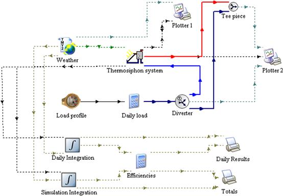
FIGURE 11.13 Model diagram of a thermosiphon solar water-heating system in simulation studio.
More details about the TRNSYS program can be found in the program manual (Klein et al., 2010) and the paper by Beckman (1998). Numerous applications of the program are mentioned in the literature. Some typical examples are for the modeling of a thermosiphon system (Kalogirou and Papamarcou, 2000; Kalogirou, 2009), modeling and performance evaluation of solar DHW systems (Oishi and Noguchi, 2000), investigation of the effect of load profile (Jordan and Vajen, 2000), modeling of industrial process heat applications (Kalogirou, 2003a; Benz et al., 1999; Schweiger et al., 2000), and modeling and simulation of a lithium bromide absorption system (Florides et al., 2002). As an example, the results of modeling a thermosiphon system are given (Kalogirou, 2009). The system model diagram is shown in Figure 11.13 and its specifications in Table 11.18. The system monthly energy flows are shown in Figure 11.14, which includes the total radiation incident on the collector (Qins), the useful energy supplied from the collectors (Qu), the hot-water energy requirements (Qload), the auxiliary energy demand (Qaux), the heat losses from the storage tank (Qenv), and the solar fraction.
Table 11.18
Specifications of the Thermosiphon Solar Water System
| Parameter | Value |
| Collector area (m2) | 2.7 (Two panels) |
| Collector slope (°) | 40 |
| Storage capacity (l) | 150 |
| Auxiliary capacity (kW) | 3 |
| Heat exchanger | Internal |
| Heat exchanger area (m2) | 3.6 |
| Hot water demand (l) | 120 (Four persons) |
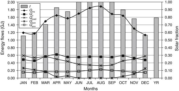
FIGURE 11.14 Energy flows of the thermosiphon solar water heater.
The system is simulated using the typical meteorological year of Nicosia, Cyprus. As it can be seen from the curve of total radiation incident on collector (Qins), the maximum value occurs in the month of August (1.88 GJ). The useful energy supplied from the collectors (Qu) is maximized in the month of April (0.62 GJ). It can be also seen from Figure 11.14 that there is a reduction in the incident solar radiation and consequently the useful energy collected during the month of May. This is a characteristic of the climatic conditions of Nicosia and is due to the development of clouds as a result of excessive heating of the ground and thus excessive convection, especially in the afternoon hours.
From the curve of the energy lost from storage tank (Qenv), it can be seen that, during the summer months, the energy lost from storage to surroundings is maximized. This is true because, in these months, the temperature in the storage tank is higher and consequently more energy is lost.
Referring to the curve of hot water load (Qload), there is a decrease of hot-water load demand during the summer months. This is attributed to the fact that, during the summer months, the total incidence of solar radiation is higher, which results to higher temperatures in the cold water storage tank (located on top of the solar collector). Consequently, the hot water demand from the hot-water storage tank during these months is reduced.
The variation in the annual solar fraction is also shown in Figure 11.14. The solar fraction, f, is a measure of the fractional energy savings relative to that used for a conventional system. As can be seen, the solar fraction is lower in the winter months and higher, reaching 100%, in the summer months. The annual solar fraction is determined to be 79% (Kalogirou, 2009).
11.5.2 WATSUN simulation program
WATSUN simulates active solar energy systems and was developed originally by the Watsun Simulation Laboratory of the University of Waterloo in Canada in the early 1970s and 1980s (WATSUN, 1996). The program fills the gap between simpler spreadsheet-based tools used for quick assessments and the more complete, full simulation programs that provide more flexibility but are harder to use. The complete list of systems that can be simulated by the original program is as follows:
• Domestic hot water system with or without storage and heat exchanger.
• Domestic hot water system with stratified storage tank.
• Phase change system, for boiling water.
• Sun switch system, stratified tank with heater.
• Swimming pool-heating system (indoor or outdoor).
• Industrial process heat system, reclaim before collector.
• Industrial process heat system, reclaim after collector.
• Industrial process heat system, reclaim before collector with storage.
• Industrial process heat system, reclaim after collector with storage.
• Variable volume tank-based system.
• Space heating system for a one-room building.
Recently, Natural Resources Canada (NRCan) developed a new version of the program, WATSUN 2009 (NRCan, 2009). This is also used for the design and simulation of active solar energy systems and is provided free from the NRCan website (NRCan, 2009). The two programs share the same name, focus on the hourly simulation of solar energy systems, and use similar equations for modeling some components; however, the new program was redeveloped from scratch, in C++, using object-oriented techniques.
The program currently models two kinds of systems: solar water-heating systems without storage and solar water-heating systems with storage. The second actually covers a multitude of system configurations, in which the heat exchanger can be omitted, the auxiliary tank-heater can be replaced with an inline heater, and the preheat tank can be either fully mixed or stratified. Simple entry forms are used, where the main parameters of the system (collector size and performance equation, tank size, etc.) can be entered easily. The program simulates the interactions between the system and its environment on an hourly basis. This can sometimes, however, break down into sub-hourly time steps, when required by the numerical solver, usually when on–off controllers change state. It is a ready-made program that the user can learn and operate easily. It combines collection, storage, and load information provided by the user with hourly weather data for a specific location and calculates the system state every hour. WATSUN provides information necessary for long-term performance calculations. The program models each component in the system, such as the collector, pipes, and tanks, individually and provides globally convergent methods to calculate their state.
WATSUN uses weather data, consisting of hourly values for solar radiation on the horizontal plane, dry bulb ambient temperature, and in the case of unglazed collectors, wind speed. At the moment, WATSUN TMY files and comma or blank delimited ASCII files are recognized by the program.
The WATSUN simulation interacts with the outside world through a series of files. A file is a collection of information, labeled and placed in a specific location. Files are used by the program to input and output information. One input file, called the simulation data file, is defined by the user. The simulation program then produces three output files: a listing file, an hourly data file, and a monthly data file.
The system is an assembly of collection devices, storage devices, and load devices that the user wants to assess. The system is defined in the simulation data file. The file is made up of data blocks that contain groups of related parameters. The simulation data file controls the simulation. The parameters in this file specify the simulation period, weather data, and output options. The simulation data file also contains information about the physical characteristics of the collector, the storage device(s), the heat exchangers, and the load.
The outputs of the program include a summary of the simulation as well as a file containing simulation results summed by month. The monthly energy balances of the system include solar gains, energy delivered, auxiliary energy, and parasitic gains from pumps. This file can be readily imported into spreadsheet programs for further analysis and plotting graphs. The program also gives the option to output data on an hourly or even sub-hourly basis, which gives the user the option to analyze the result of the simulation in greater detail and facilitates comparison with monitored data, when these are available.
Another use of the program is the simulation of active solar energy systems for which monitored data are available. This can be done either for validation purposes or to identify areas of improvement in the way the system works. For this purpose, WATSUN allows the user to enter monitored data from a separate file, called the alternate input file. Monitored climatic data, energy collected, and many other data can be read from the alternate input file and override the values normally used by the program. The program can also print out strategic variables (such as collector temperature or the temperature of water delivered to the load) on an hourly basis for comparison with monitored values.
The program was validated against the TRNSYS program using several test cases. Program-to-program comparisons with TRNSYS were very favorable; differences in predictions of yearly energy delivered were less than 1.2% in all configurations tested (Thevenard, 2008).
11.5.3 Polysun simulation program
The Polysun program provides dynamic annual simulations of solar thermal systems and helps to optimize them (Polysun, 2008). The program is user-friendly and the graphical user interface permits comfortable and clear input of all system parameters. All aspects of the simulation are based on physical models that work without empirical correlation terms. The basic systems that can be simulated include:
The input of the required data is very easy and done in a ready-made graphical environment like the one shown in Figure 11.15. The input of the various parameters for each component of the system can be done by double-clicking on each component. Such templates are available for all types of systems that can be modeled with Polysun, and there is a template editor for users who want to create their own, tailored to the requirements of specific products. The modern and appealing graphical user interface makes it easy and fast to access the software. The convenient modular unit construction system allows the combination and parameterization of different system components through simple menu prompts.
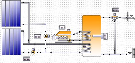
FIGURE 11.15 Polysun graphical environment.
Polysun is now in version 5.10 and makes the design of solar thermal systems simple and professional. An earlier version of Polysun was validated by Gantner (2000) and found to be accurate to within 5–10%. The characteristics of the various components of the system can be obtained from ready-made catalogs, which include a large variety of market available components, but the user can add also the characteristics of a component, such as a collector, not included in the catalogs. The components included in catalogs comprise storage tanks, solar collectors, pipes, boilers, pumps, heat exchangers, heat pumps, buildings, swimming pools, PV modules and inverters, and many more. The program also features simple analysis and evaluation of simulations through graphics and reports. Worldwide meteorological data for 6300 locations are available, and new locations can be individually defined. There is also provision to specify the temperature of cold water and of the storage room. All features of the program are given in English, Spanish, Portuguese, French, Italian, Czech, and German.
Storage tanks can be specified with up to 10 connection ports, up to six internal heat exchangers, up to three internal heaters, and an internal tank and coil heat exchanger. The output of the program includes solar fraction, energy values (on the loop and component levels), temperatures, flow rate, and status for all components as a curve diagram, economic analysis, and summary of the most relevant values as a PDF file.
The simulation algorithm provides dynamic simulation, including variable time steps, flow rate calculation including consideration of pressure drop, and material properties depending on temperature.
Leave a Reply